[Hands-On] Head-based Sound Classification using ViT

Head-based Sound Classification using ViT (Image by the author using ChatGPT)

(You can find the Korean version of the post at this link.)

This post is the third tutorial in our series on head-based classification techniques. In the previous post, we examined head-based classification in texts and images.

[embed][Hands-On] Head-based Text Classification with BERT Explore BERT for text classification with our tutorial on head-based methods, ideal for understanding and implementing…medium.com

[embed][Hands-On] Head-based Image Classification with ViT Explore head-based image classification with Vision Transformers. Learn how ViT applies to image patches for object…medium.com

In this tutorial, we’ll explore how to use a Vision Transformer (ViT) model for sound classification. While ViT was originally designed for image classification tasks, we’ll adapt it to classify sounds by converting audio data into visual representations called spectrograms.

In our previous post, we explored various methods of converting sound into images. In this post, we plan to use one of those methods, specifically the mel-spectrogram technique, to transform audio into images. We will then utilize a well-known image recognition tool, the Vision Transformer (ViT), to perform recognition on these transformed images.

We’ll use the UrbanSound8K dataset, which contains various urban sound recordings, to train our model.

Here’s what we’ll cover:

1. Converting sound data into Mel-spectrograms
2. Adapting the ViT model to handle these spectrograms
3. Training the model on a subset of the UrbanSound8K dataset
4. Evaluating the model’s performance and visualizing the results

Let’s dive in!

1. Setting Up the Environment

First, let’s install the necessary libraries and check if a GPU is available:

!pip install -qq librosa seaborn transformers datasets

import torch
print("GPU available:", torch.cuda.is_available())

2. Loading the UrbanSound8K Dataset

We’ll use the Hugging Face Datasets library to load our data:

from datasets import load_dataset

dataset = load_dataset("danavery/urbansound8K")
print(dataset)

DatasetDict({
    train: Dataset({
        features: ['audio', 'slice_file_name', 'fsID', 'start', 'end', 'salience', 'fold', 'classID', 'class'],
        num_rows: 8732
    })
})

The UrbanSound8K dataset is a collection of urban sound recordings widely used in acoustic scene classification and environmental sound recognition research.

Here are its key features:

1. Content: It contains 8,732 labeled sound excerpts of urban sounds from 10 classes.
2. Classes: The dataset includes the following urban sound categories:

• Air conditioner
• Car horn
• Children playing
• Dog bark
• Drilling
• Engine idling
• Gun shot
• Jackhammer
• Siren
• Street music

3. Splitting the Dataset

Let’s split our dataset into training and validation sets:

USE_FULL_DATA = True

if USE_FULL_DATA:
    train_test_split = dataset['train'].train_test_split(test_size=0.2, seed=42)
else:
    # Set the fraction of the dataset to use (e.g., 10%)
    fraction = 0.1

    # Sample a smaller subset of the dataset
    small_dataset = dataset['train'].shuffle(seed=42).select(range(int(len(dataset['train']) * fraction)))

    # Split the smaller dataset into train (80%) and validation (20%) sets
    train_test_split = small_dataset.train_test_split(test_size=0.2, seed=42)  # <-- small dataset

train_dataset = train_test_split['train']
valid_dataset = train_test_split['test']

The entire dataset is very large. If you want to quickly run through the entire code, you can set USE_FULL_DATA=False.

4. Data Preprocessing

Now comes the crucial part: converting our audio data into Mel-spectrograms.

We’ll use the torchaudio library for this:

import torch
import torchaudio
from torchaudio.transforms import MelSpectrogram, Resample
from torchvision.transforms import Resize, Normalize

# Define Mel Spectrogram transformation with adjusted n_mels
sample_rate = 22050
n_mels = 64  # Adjusted from 128 to 64 to avoid the warning
mel_spectrogram = MelSpectrogram(
    sample_rate=sample_rate,
    n_mels=n_mels
)

# Define resizing and normalization transformations
resize = Resize((224, 224))
normalize = Normalize(mean=[0.5], std=[0.5])

# Define a preprocessing function with data type consistency
def preprocess(example):
    audio = example['audio']['array']
    # Convert audio to a FloatTensor to match kernel dtype
    audio = torch.tensor(audio, dtype=torch.float32)
    # Resample if needed
    if example['audio']['sampling_rate'] != sample_rate:
        resample = Resample(orig_freq=example['audio']['sampling_rate'], new_freq=sample_rate)
        audio = resample(audio)

    # Generate Mel Spectrogram
    mel_spec = mel_spectrogram(audio)
    mel_spec = mel_spec.unsqueeze(0)  # (1, n_mels, time)

    # Convert to image and normalize
    mel_spec = resize(mel_spec)
    mel_spec = normalize(mel_spec)

    # Convert label to tensor
    label = torch.tensor(example['classID'], dtype=torch.long)

    return {'image': mel_spec, 'label': label}

# Apply preprocessing to train and validation datasets
train_dataset = train_dataset.map(preprocess, remove_columns=['audio', 'slice_file_name', 'fsID', 'start', 'end', 'salience', 'fold', 'class'], batched=False)
valid_dataset = valid_dataset.map(preprocess, remove_columns=['audio', 'slice_file_name', 'fsID', 'start', 'end', 'salience', 'fold', 'class'], batched=False)

# Extract unique class IDs from the train dataset to determine the number of classes
num_labels = len(set(train_dataset['label']))

print(f"Number of classes: {num_labels}")

Number of classes: 10

5. Visualizing a Sample Mel Spectrogram

Let’s visualize one of our processed spectrograms:

from IPython.display import Audio, display

sample = dataset['train'][0]
# Extract the audio array and sampling rate
audio_array = sample['audio']['array']
sampling_rate = sample['audio']['sampling_rate']

# Extract the audio array and sampling rate
audio_array = sample['audio']['array']
sampling_rate = sample['audio']['sampling_rate']

# Display audio player
print("Audio Player:")
display(Audio(audio_array, rate=sampling_rate))

import numpy as np
import matplotlib.pyplot as plt

# Select a sample from the training dataset
sample = preprocess(sample)

# Access the tensor
mel_spec = sample['image'][0]

# Plot the Mel Spectrogram
plt.figure(figsize=(10, 4))
plt.imshow(mel_spec, aspect='auto', origin='lower')
plt.title('Mel Spectrogram of a Sample from UrbanSound8K')
plt.xlabel('Time')
plt.ylabel('Mel Frequency')
plt.colorbar(format='%+2.0f dB')
plt.show()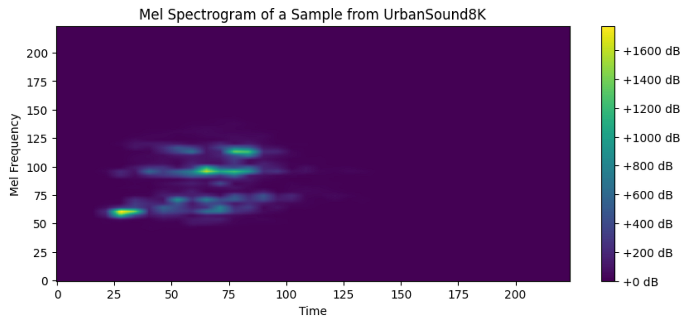

Mel Spectrogram of a Sample from UrbanSound8K

This gives us a visual representation of how our audio data looks after preprocessing.

6. Preparing the DataLoader

We’ll use PyTorch’s DataLoader to efficiently load our data during training:

from torch.utils.data import DataLoader

# Create DataLoader for training and validation
train_loader = DataLoader(train_dataset, batch_size=32, shuffle=True)
valid_loader = DataLoader(valid_dataset, batch_size=32, shuffle=False)

7. Defining the Vision Transformer (ViT) Model

Now, let’s set up our ViT model:

from transformers import ViTForImageClassification

# Define the Vision Transformer model using the calculated num_labels
model = ViTForImageClassification.from_pretrained(
    'google/vit-base-patch16-224',
    num_labels=num_labels,
    ignore_mismatched_sizes=True  # Add this parameter to handle the size mismatch
)

# Move the model to GPU if available
model = model.to('cuda' if torch.cuda.is_available() else 'cpu')

Head-based Classification: The Vision Transformer model we’re using employs a head-based classification approach. In this context, the “head” refers to the final layers of the network that perform the actual classification task. The base ViT model extracts features from the input images, and the classification head uses these features to make predictions.

By setting num_labels=num_labels in the model initialization, we're actually customizing the classification head of the ViT model. This parameter tells the model how many classes it needs to predict, and the library automatically adds a final linear layer (the classification head) with the appropriate number of output neurons. For example, if num_labels is 10 (as in our UrbanSound8K dataset), the final layer will have 10 output neurons, each corresponding to one of our sound classes. This allows the model to output probabilities for each of the 10 classes when making predictions.

Another important thing to note : ViT typically expects 3-channel (R,G,B) input images. However, our spectrogram, while appearing colorful when visualized, is actually a single-channel (grayscale) image. The colors you see are just a representation of intensity values. To use this with ViT, we’ll need to artificially expand our 1-channel spectrogram into a 3-channel image during training and prediction. We will explore the expanding trick later.

8. Training the Model

Let’s define our loss function and optimizer:

import torch.optim as optim

# Define loss function and optimizer
criterion = torch.nn.CrossEntropyLoss()
optimizer = optim.Adam(model. Parameters(), lr=1e-4)

Now, we can train our model:

# Define the training function
def train(model, loader, criterion, optimizer, device, log_interval=10):
    model.train()
    running_loss = 0.0
    total = 0
    correct = 0

    for idx, batch in enumerate(loader):
        # Convert list of tensors to a single tensor
        if isinstance(batch['image'], list):
            batch['image'] = torch.tensor(np.array(batch['image'])).permute(3, 0, 1, 2)
            batch['image'] = batch['image'].repeat(1, 3, 1, 1)  # since spectrogram has 1 channel

        images = batch['image'].to(device)
        labels = batch['label'].to(device)

        optimizer.zero_grad()
        outputs = model(images).logits
        loss = criterion(outputs, labels)
        loss.backward()
        optimizer.step()

        running_loss += loss.item() * images.size(0)

        # Calculate the number of correct predictions
        _, predicted = torch.max(outputs, 1)
        total += labels.size(0)
        correct += (predicted == labels).sum().item()

        # Log the progress at every `log_interval` batches
        if idx % log_interval == 0:
            print(f"Batch {idx}/{len(loader)}, Loss: {loss.item():.4f}, Accuracy: {100 * correct / total:.2f}%")

    epoch_loss = running_loss / len(loader.dataset)
    epoch_accuracy = 100 * correct / total
    return epoch_loss, epoch_accuracy

# Define the validation function
def validate(model, loader, criterion, device):
    model.eval()
    running_loss = 0.0
    correct = 0
    total = 0

    all_labels = []
    all_predictions = []

    with torch.no_grad():
        for batch in loader:
            # Convert list of tensors to a single tensor
            if isinstance(batch['image'], list):
                batch['image'] = torch.tensor(np.array(batch['image'])).permute(3, 0, 1, 2)
                batch['image'] = batch['image'].repeat(1, 3, 1, 1)  # since spectrogram has 1 channel

            images = batch['image'].to(device)
            labels = batch['label'].to(device)

            outputs = model(images).logits
            loss = criterion(outputs, labels)
            running_loss += loss.item() * images.size(0)

            _, predicted = torch.max(outputs, 1)
            total += labels.size(0)
            correct += (predicted == labels).sum().item()

            all_labels.extend(labels.cpu().numpy())
            all_predictions.extend(predicted.cpu().numpy())

    epoch_loss = running_loss / len(loader.dataset)
    accuracy = 100 * correct / total
    return epoch_loss, accuracy, all_labels, all_predictions

# Train and validate the model
device = 'cuda' if torch.cuda.is_available() else 'cpu'
num_epochs = 10

for epoch in range(num_epochs):
   train_loss, train_accuracy = train(model, train_loader, criterion, optimizer, device)
   valid_loss, valid_accuracy, all_labels, all_predictions = validate(model, valid_loader, criterion, device)
   print(f'Epoch {epoch+1}/{num_epochs}, Train Loss: {train_loss:.4f}, Train Accuracy: {train_accuracy:.2f}%, Validation Loss: {valid_loss:.4f}, Validation Accuracy: {valid_accuracy:.2f}%')

Batch 0/219, Loss: 2.3437, Accuracy: 9.38%
Batch 10/219, Loss: 2.1411, Accuracy: 24.72%
Batch 20/219, Loss: 1.7757, Accuracy: 32.14%
Batch 30/219, Loss: 1.1317, Accuracy: 38.51%
Batch 40/219, Loss: 0.8994, Accuracy: 43.22%
Batch 50/219, Loss: 1.2490, Accuracy: 46.38%
Batch 60/219, Loss: 0.8936, Accuracy: 50.26%
Batch 70/219, Loss: 0.7673, Accuracy: 52.42%
Batch 80/219, Loss: 0.7324, Accuracy: 55.29%
Batch 90/219, Loss: 0.8253, Accuracy: 57.45%
Batch 100/219, Loss: 0.6350, Accuracy: 59.22%
Batch 110/219, Loss: 0.5952, Accuracy: 61.26%
Batch 120/219, Loss: 0.7226, Accuracy: 62.60%
Batch 130/219, Loss: 0.4664, Accuracy: 63.72%
Batch 140/219, Loss: 0.8109, Accuracy: 64.80%
Batch 150/219, Loss: 0.9543, Accuracy: 65.91%
Batch 160/219, Loss: 0.2443, Accuracy: 67.10%
Batch 170/219, Loss: 0.7276, Accuracy: 67.60%
Batch 180/219, Loss: 0.5884, Accuracy: 68.46%
Batch 190/219, Loss: 0.5761, Accuracy: 69.19%
Batch 200/219, Loss: 0.5276, Accuracy: 69.88%
Batch 210/219, Loss: 0.8075, Accuracy: 70.68%
Epoch 1/10, Train Loss: 0.8661, Train Accuracy: 71.25%, Validation Loss: 0.5469, Validation Accuracy: 82.83%
...
...
Batch 80/219, Loss: 0.0472, Accuracy: 97.99%
Batch 90/219, Loss: 0.0405, Accuracy: 98.08%
Batch 100/219, Loss: 0.0026, Accuracy: 98.17%
Batch 110/219, Loss: 0.0420, Accuracy: 98.28%
Batch 120/219, Loss: 0.0029, Accuracy: 98.40%
Batch 130/219, Loss: 0.0012, Accuracy: 98.47%
Batch 140/219, Loss: 0.0237, Accuracy: 98.52%
Batch 150/219, Loss: 0.0012, Accuracy: 98.59%
Batch 160/219, Loss: 0.0281, Accuracy: 98.64%
Batch 170/219, Loss: 0.0410, Accuracy: 98.67%
Batch 180/219, Loss: 0.0643, Accuracy: 98.67%
Batch 190/219, Loss: 0.0237, Accuracy: 98.72%
Batch 200/219, Loss: 0.0553, Accuracy: 98.74%
Batch 210/219, Loss: 0.0382, Accuracy: 98.79%
Epoch 10/10, Train Loss: 0.0370, Train Accuracy: 98.75%, Validation Loss: 0.4199, Validation Accuracy: 89.64%

In the code above, you can see that we use batch['image'].repeat(1, 3, 1, 1) to forcibly set the number of channels to 3. For higher performance, it could be tuned in a more elegant and precise manner, but here, we have implemented it in a very simple way

This training used the full dataset, and after about 10 epochs of training, we achieved a classification accuracy of around 89% on the validation data.

9. Evaluating the Model

After training, let’s evaluate our model using precision, recall, F1-score, and visualize the confusion matrix:

label_map = {
    0: "air_conditioner",
    1: "car_horn",
    2: "children_playing",
    3: "dog_bark",
    4: "drilling",
    5: "engine_idling",
    6: "gun_shot",
    7: "jackhammer",
    8: "siren",
    9: "street_music"
}

# convert label-ids to texts
all_labels_text = [label_map[label] for label in all_labels]
all_predictions_text = [label_map[pred] for pred in all_predictions]

from sklearn.metrics import classification_report, confusion_matrix
import seaborn as sns
import matplotlib.pyplot as plt

# Generate classification report using text labels
report = classification_report(all_labels_text, all_predictions_text, target_names=list(label_map.values()))
print("Classification Report:\n", report)

# Compute confusion matrix using text labels
conf_matrix = confusion_matrix(all_labels_text, all_predictions_text, labels=list(label_map.values()))

# Plot confusion matrix
plt.figure(figsize=(10, 8))
sns.heatmap(conf_matrix, annot=True, fmt='d', cmap='Blues', xticklabels=list(label_map.values()), yticklabels=list(label_map.values()))
plt.title('Confusion Matrix')
plt.xlabel('Predicted Label')
plt.ylabel('True Label')
plt.show()

Classification Report:
                   precision    recall  f1-score   support

 air_conditioner       0.95      0.96      0.95       207
        car_horn       0.84      0.85      0.85        81
children_playing       0.86      0.81      0.84       192
        dog_bark       0.92      0.82      0.86       211
        drilling       0.95      0.84      0.89       205
   engine_idling       0.95      0.95      0.95       209
        gun_shot       0.99      1.00      0.99        74
      jackhammer       0.92      0.94      0.93       189
           siren       0.91      0.91      0.91       194
    street_music       0.74      0.94      0.83       185

        accuracy                           0.90      1747
       macro avg       0.90      0.90      0.90      1747
    weighted avg       0.90      0.90      0.90      1747

Confusion Matrix of Head-Based Sound Classification — UrbanSound8K

When using the full dataset, we can see that the model achieves an f1-score of 0.90. Interestingly, we can observe that the trained model often gets confused between certain classes, such as ‘children_playing’ and ‘street_music’, or ‘drilling’ and ‘jackhammer’.

10. Making Predictions

Finally, let’s use our trained model to make predictions on a single sound sample:

# Select a random sample from the validation set
sample_idx = 0
sample = valid_dataset[sample_idx]

# Make prediction
model.eval()
with torch.no_grad():
    sample['image'] = torch.tensor(np.array( [sample['image']]))
    sample['image'] = sample['image'].repeat(1, 3, 1, 1)  # since spectrogram has 1 channel
    print( sample['image'].shape )

    image = sample['image'].to(device)
    output = model(image).logits
    _, predicted_label = torch.max(output, 1)

actual_label_text = label_map[sample["label"]]
predicted_label_text = label_map[predicted_label.item()]

print(f'Actual Label: {actual_label_text}, Predicted Label: {predicted_label_text}')

Actual Label: children_playing, Predicted Label: children_playing

Conclusion

In this tutorial, we successfully addressed the sound classification problem using the Vision Transformer (ViT) model. We transformed audio data into mel-spectrograms, converting them into images, and then trained the ViT model to effectively classify urban sounds based on these visual representations.

This approach demonstrates how converting sound into images allows us to apply existing image classification models directly to sound recognition tasks. It’s important to note that this method isn’t limited to ViT; any form of image classification technique can be applied.

For those looking to delve deeper, experimenting with different audio preprocessing techniques, exploring alternative image architectures, or utilizing different datasets can further enhance performance.

You can run the code discussed in this post directly via the link below.

[embed][Hands-On] Head-based Sound Classification using ViT Hugman Sangkeun Jungcolab.research.google.com

In the next article, we will explore how to perform prompt-based classification on the same sound classification problem using a model called CLAP.

[embed][Hands-On] Prompt-based Sound Classification with CLIP Implementing Prompt-Based Sound Classification with CLAPmedium.com