How many licences should you commit to before the rollout has started?

I built an open-source model for that decision and tested it against a public software licensing audit

Enterprise software buying contains one decision that is harder than it looks:

How much should a buyer commit before the organization is actually ready to deploy?

Commit more and the supplier may cut the unit price. Commit less and the buyer may lose volume discounts, budget predictability, or enterprise rights. The commercial decision is made at signature. The value only appears if infrastructure, integrations, security approvals, data, delivery teams, and users are ready on time.

That timing mismatch is not ordinary shelfware. Shelfware gets discovered after purchase. This is a pre-award sourcing problem: choosing a commitment shape before anyone knows how adoption will actually go.

I built an open-source Software Commitment and Ramp Optimizer to make that decision explicit. It models uncertain adoption, applies real commercial mechanics month by month, tests alternative negotiation policies, measures tail risk, and calculates how much a buyer could rationally pay for flexibility.

I used a City of Toronto Auditor General report as the public test case because it contains unusually concrete deployment and cost data. This is not a claim that the City could have bought the counterfactual terms, and it is not a retrospective savings estimate. It is a reproducible experiment showing what a sourcing team could have quantified before committing.

Independence and evidence note: This project is independent and is not affiliated with or endorsed by the City of Toronto, Microsoft, SAP, or ForgeRock. Published audit facts are separated from derived values and illustrative model assumptions throughout the repository.

The Toronto case: deployment did not match the commitment clock

Toronto's Auditor General published Audit of Software Acquisition and Licence Management: Managing and Optimizing Value from Software Licences in December 2024.

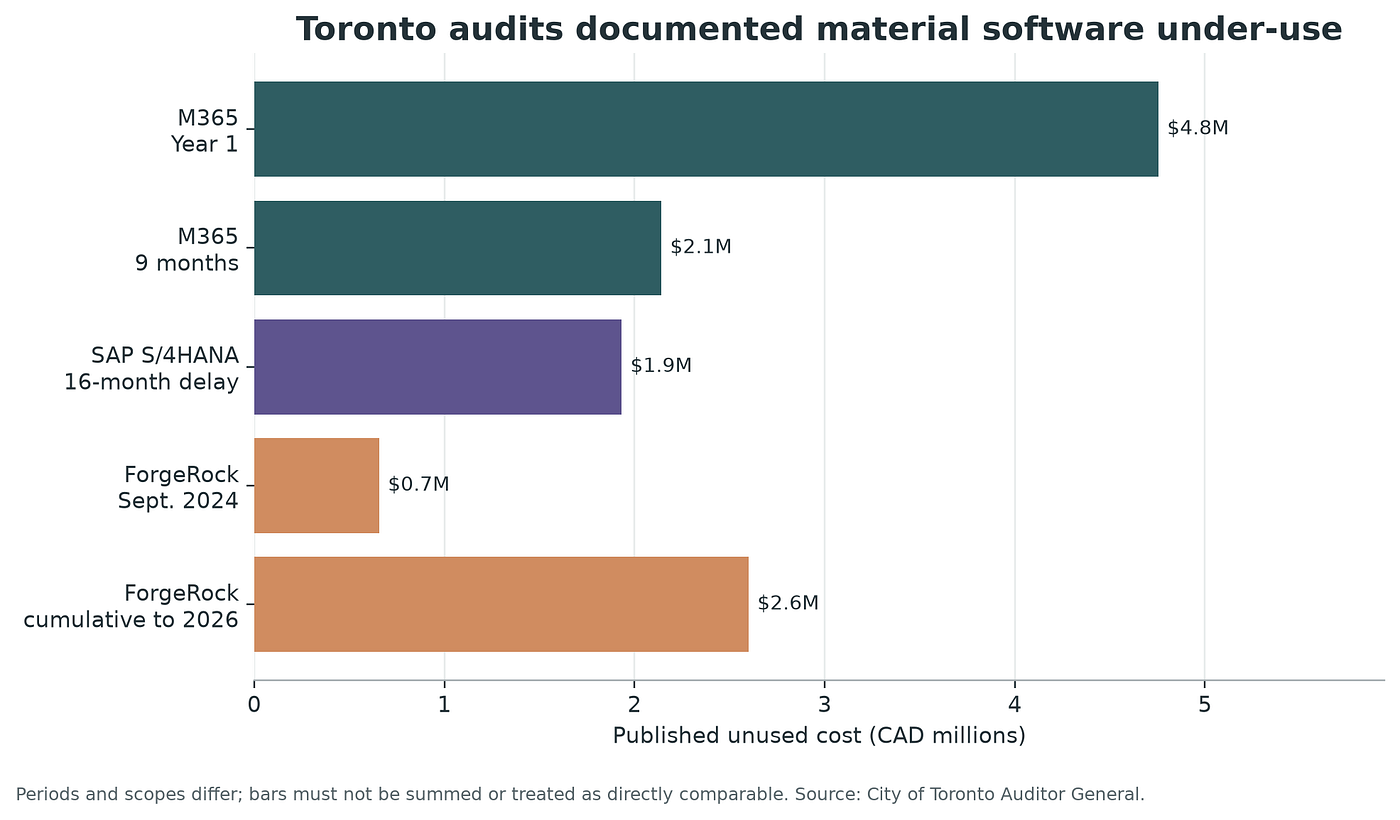
For Microsoft 365, the audit described an agreement covering 10,000 enterprise users and two add-ons as 30,000 subscription licences. The published annual subscription cost was CAD 5,140,800.

At the end of the first agreement year, deployment was 7.5%, and the audit reported CAD 4,755,240 in unused subscription cost. During the first nine months of the second year, usage was reported at 44.5%, with CAD 2,141,357 in unused subscription cost.

The report documented similar patterns elsewhere in the software portfolio. It reported CAD 1,932,376 associated with unused SAP S/4HANA licences and related services during a 16-month project delay. For ForgeRock, it reported 15,331 of 800,000 purchased units in use as of September 2024, and CAD 657,177 in unused cost. A 2026 follow-up report later reported 45,117 units in use, a contractual purchase of at least 700,000 annually, and cumulative unused cost of CAD 2.6 million since project inception.

Those periods and scopes are different. I do not add them together and I do not treat the bars as direct comparisons. What they establish is that the problem is real: software commercial commitments and implementation readiness can run on different clocks.

There is an important counterpoint. City management reported volume-discount savings associated with the M365 agreement. So the analytical question is not whether volume commitments are bad. They are not. The question is narrower:

At what price does the discount stop compensating for the risk of paying before activation?

You can calculate that. It is a break-even problem.

What an optimizer could have changed

The audit describes an outcome. A sourcing tool has to act earlier than that.

Before signature, a buyer usually has at least five imperfect inputs: a target population, a deployment plan, known technical and organizational dependencies, supplier pricing for one or more commitment levels, and whatever flexibility terms are available, even if they carry a premium.

The interface does not ask the buyer to translate those facts into Monte Carlo or CVaR parameters. It asks plain-language commercial questions, then five evidence-gate questions about demand, architecture, delivery, dependencies, and usage reporting. A translation layer maps the commercial answers into the numerical model. The gate decides whether the output can be treated as an approvable commitment.

Buyers rarely know one correct deployment forecast. What they can know is a range: earliest, most likely, and latest readiness; possible final demand; and how fast adoption might grow after a delay.

The optimizer converts those uncertainties into thousands of plausible monthly demand paths, then prices the same paths under different commercial structures: full commitment at commencement, phased activation, monthly through annual review cadences, true-up only or true-up with true-down, minimum floors, operational buffers, overage pricing, fixed and one-time fees, annual escalation, and an explicit unit-price premium for flexibility.

Instead of arguing abstractly that a phased ramp should save money, the sourcing team can say something a supplier has to respond to:

With these delivery assumptions and this risk tolerance, semiannual activation remains economically preferable up to a unit price of X. Above X, the upfront alternative becomes better. Here is the overage exposure and P90 budget for each option.

Could this have prevented Toronto's unused M365 cost?

Not automatically, no. A model cannot force an organization to use it, a supplier to offer flexible billing, or a decision-maker to turn down a bulk discount. The public record also does not disclose the complete contract, the internal forecast, the bundle value, or every concession available at signature.

But the audit contains one fact that should have changed the approval process before any simulation was run: the network had been estimated to support only 6,000 users, while the agreement covered an initial 10,000 users, and architecture scalability still required review.

So the improved application adds a readiness gate that does not compensate. It asks whether demand is evidenced, technical capacity is confirmed, a dated deployment plan is approved, critical dependencies are cleared, a required pilot is complete, monthly usage reporting exists, and an owner is assigned. If architecture is not confirmed, good answers elsewhere cannot average the problem away. The result is:

Hold the full commitment. The modelled quantity may be used for planning, but it is not an approved purchase-order quantity until the blocker is closed or an authorized exception is documented.

If that control had been completed honestly and enforced, a 10,000-user full commitment would not have passed as an ordinary approval. The next steps would have been to identify the independently verified first deployable wave; ask suppliers to price the full commitment, phased activation, and phased activation with true-down on one comparable schedule; evaluate total and P90 cost rather than headline unit discount alone; put activation dates, quantity formula, usage evidence, delay rights, and repricing limits into the order form; and block each later purchase order until deployment and active-use evidence has been reviewed.

A decision-maker could still choose the full commitment. The difference is that the architecture gap, the unused-cost exposure, the owner, the rejected phased alternative, and the override would all be visible in the approval record.

The audit examined CAD 8,996,400 of M365 subscription spend across Year 1 and the first nine months of Year 2, and reported CAD 6,896,597 of unused cost. Management reported approximately CAD 2.8 million of bulk-discount savings over the five-year contract. The early unused cost therefore exceeded that stated five-year discount by about CAD 4.10 million.

The application includes a separate retrospective slider. It subtracts the published unused cost from examined spend to create a used-cost proxy, then applies an illustrative premium for usage-aligned billing. At a 15% premium, the proxy is:

examined spend                         CAD 8,996,400
less audit-reported unused cost        CAD 6,896,597
used-cost proxy                        CAD 2,099,803
usage-aligned proxy at 15% premium     CAD 2,414,773
upper-bound difference                 CAD 6,581,627

That is not a savings claim. It uses observed outcomes, it assumes billing could have followed use, and it ignores confidential bundle value and supplier constraints. Its purpose is to show the scale of the negotiation boundary, and why deployment-aligned pricing deserved a mandatory response rather than a polite one.

The tool, component by component

The code is deliberately transparent. There is no proprietary optimization service and no language model making hidden commercial judgments.

1. Evidence boundary and case loader

The first component prevents a common research error: blending public facts and invented counterfactuals in the same table.

The Toronto case stores published audit facts in a CSV with page references, derived arithmetic under a distinct label, simulation assumptions in a JSON configuration, and source URLs in a dedicated source note.

Typed models validate every configuration. Negative fees, unsorted price tiers, impossible delay ranges, and invalid probabilities all fail before the simulation begins.

This component does not optimize anything. Its job is epistemic: make it obvious what is known, what is calculated, what is assumed, and what the user entered.

2. Adoption forecast

The forecast engine builds a smooth logistic rollout between an initial active population and a final target. It is normalized so month zero matches the day-one population, the target is reached at the configured rollout-completion month, and demand holds at that level for the rest of the contract.

Each Monte Carlo scenario varies three things: final demand, because the target population may change; adoption speed, because rollout can run faster or slower; and delay, because infrastructure or implementation dependencies can shift the whole adoption curve to the right.

Delay uses a triangular distribution. That is deliberately modest. A sourcing team often cannot estimate a sophisticated distribution, but it can agree on an earliest, most likely, and latest delay. The random seed is fixed, so another reviewer can reproduce the same paths.

3. Commercial-term model

A commercial option is a data object, not a hard-coded formula. It holds price tiers, initial commitment, contractual floor, review cadence, true-down rights, buffer, overage multiplier, fees, escalation, and flexibility premium.

That is what makes the model usable in an RFP or a negotiation. An analyst can replace illustrative terms with the actual rows from supplier bids without touching the engine.

4. Monthly pricing engine

For every demand path, the pricing engine establishes the initial commitment:

initial commitment = max(contractual floor,
                         target × initial commitment percentage)

At each review date it calculates requested capacity as active demand plus a buffer. A true-up-only option can increase but cannot reduce the baseline. A true-down option can move in either direction, subject to the floor.

If demand exceeds commitment between review dates, the excess is recorded as emergency overage and billed at its configured multiplier. This matters, because an optimizer can otherwise produce a superficially cheap answer by quietly turning normal demand into exceptions.

The engine produces a monthly cash flow, unused capacity, unused cost, overage units, overage cost, and utilization for every path.

5. Monte Carlo evaluator

One forecast is fragile. The evaluator applies each commercial option to every demand scenario and reports a distribution of outcomes: expected cost, median cost, P90 cost, 90% conditional value at risk (CVaR), unused cost and unit-months, overage cost and unit-months, and utilization.

P90 is the cost not exceeded in 90% of simulations. CVaR is the average cost among the costliest 10%. That second number is useful because two options can have similar averages and very different budget exposure in the tail.

6. Risk-adjusted objective

The default ranking metric is:

risk-adjusted cost = expected cost
                   + 0.25 × (CVaR90 − expected cost)

The 0.25 is not a universal truth. It says this example gives some weight, but not dominant weight, to costly tail outcomes. The guided interface asks whether the organization is cost focused, balanced, or conservative, then maps that answer to documented risk and overage settings. Advanced users can still inspect the underlying metrics.

7. Policy optimizer

The search is an auditable grid, not a black box. It tests combinations of initial commitment percentage, buffer, review frequency, and true-down permission.

More frequent review and true-down carry configurable price premiums. In the Toronto experiment, the default search prices monthly review at 20%, quarterly at 12%, semiannual at 6%, and annual at 0%. True-down adds 8%.

The optimizer also enforces a feasibility constraint: expected emergency-overage unit-months cannot exceed 10% of expected consumed unit-months. I added that after the first run produced a cheap but commercially weak answer that leaned heavily on overage. That failure was worth having. An optimizer will exploit whatever model you give it, so the operational constraints have to be in the model.

8. Break-even premium calculator

The most valuable output may be a boundary rather than a winning policy.

The calculator reprices the flexible policy repeatedly until its risk-adjusted cost equals the locked baseline. It answers how much extra unit price the buyer could absorb for the activation rights before the economics reverse.

That can become an RFP evaluation rule or a negotiation walk-away point. It does not predict what a supplier will quote.

9. Approval, sourcing, and control workflow

The Streamlit interface is built as a procurement operating workflow rather than a model console. The first tab asks for information that procurement, software asset management, architecture, and the project team can reasonably provide. It returns the number of licence units to order at contract start, the usage-review cadence and phase-by-phase expected buying schedule, the formula to apply when actual usage replaces the forecast at each review, a financial comparison with full upfront commitment, the maximum modelled price premium to consider for flexibility, supplier terms to request and actions to complete before issuing the purchase order, a downloadable Markdown procurement plan, and detailed JSON for reviewers who want the assumptions and model outputs.

The second tab compares actual supplier offers. Analysts enter each offer's unit price, starting quantity, floor, review cadence, true-down right, buffer, overage, escalation, and fees. Every offer is evaluated on the same seeded demand paths.

The third tab is post-award. It takes committed units, active use, assigned-but-inactive units, price, buffer, and true-down permission, then calculates current unused exposure and produces a reclaim, freeze, true-up, true-down, or maintain action. If the agreement has no true-down right, the tool does not invent one. It recommends consuming the existing pool and seeking credits or renewal relief.

CVaR, candidate counts, and other technical diagnostics stay available in an advanced section. The Toronto evidence sits in its own tab, so public facts, prospective control logic, and retrospective counterfactuals do not get confused with each other.

The command-line interface creates the same reproducible result bundle for peer review or version control.

The Toronto experiment

I anchored only three numerical inputs to the M365 audit: target quantity of 30,000 licence equivalents, annual cost of CAD 5,140,800, and an initial active population of 7.5%, or 2,250.

The annual cost gives a simple allocation proxy:

CAD 5,140,800 ÷ 30,000 ÷ 12 = CAD 14.28 per unit per month

That proxy reconciles exactly with the published Year-1 result:

30,000 × CAD 14.28 × 12 = CAD 5,140,800
92.5% unused × CAD 5,140,800 = CAD 4,755,240

An automated regression test covers this arithmetic.

Everything else is marked as an assumption. The publication run uses a 36-month horizon, a month-16 expected rollout midpoint, 45% probability of a material delay, a triangular delay of 2/6/12 months, 10% final-demand volatility, 15% adoption-speed volatility, 2,000 scenarios, and a fixed seed.

I compared three named options and the optimizer: the published upfront commitment proxy, an illustrative quarterly ramp at a 15% premium, illustrative monthly true-down flexibility at a 25% premium, and the best feasible policy from the configured search.

Results: a boundary, not a savings claim

The optimizer evaluated 288 non-duplicate candidates. Of those, 204 met the 10% overage guardrail.

The lowest risk-adjusted result used a 7.5% initial floor, six-month reviews, true-up only, a 10% buffer, and a modelled 6% flexibility premium.

[embed]

The modelled risk-adjusted difference is CAD 6.39 million. I would not call that savings. Toronto did not run this model before the agreement, the alternative terms are hypothetical, the private bundle value is not known, and supplier acceptance is not known either.

The defensible interpretation is narrower:

Under the documented assumptions, the cost of timing mismatch is large enough that a phased commitment remains attractive even after charging a meaningful premium for flexibility.

The selected policy's expected overage share is 9.0%, just below the configured 10% feasibility limit. That is an exposure to manage, not a free benefit.

The break-even premium came out at roughly 78.4% above the public cost proxy. The selected policy itself only uses a 6% premium. The 78.4% figure is the point where the modelled advantage disappears. It is high because the simulated upfront policy carries substantial idle capacity during the ramp. It is not a software-market benchmark and not a recommended premium.

The ramp view shows the mechanism more clearly than the headline number does.

The upfront proxy pays for the target well before expected activation. Quarterly and semiannual policies follow adoption in steps. The optimized policy accepts some overage exposure in exchange for less stranded commitment, and the guardrail keeps that exposure inside the configured tolerance.

How this could have helped before signature

The tool would not have predicted Toronto's rollout. It could have improved the sourcing process in five concrete ways.

1. Convert readiness into a commercial schedule

Implementation milestones could have been translated into activation tranches instead of sitting in a project plan disconnected from the order form.

2. Price the discount against the delay risk

Management's reported volume discount could have been compared with the expected and tail cost of early commitment. Both sides of the trade-off would appear in one model.

3. Define negotiation asks precisely

Instead of requesting vague flexibility, the team could test specific rights: 2,250 units at commencement, protected unit pricing for later tranches, six-month measurement dates, a 10% buffer, true-up rules based on verified activation, and a cap on overage price or administrative exposure.

The supplier could reject or reprice any of those. The buyer would still know the price at which they stop being worth asking for.

4. Expose ownership of assumptions

Delivery owns the rollout range. Architecture and security own dependency risk. Finance owns budget tolerance. Procurement owns bid normalization and negotiation. Legal owns whether the measurement and adjustment clauses are enforceable. The model makes those handoffs visible.

5. Preserve a decision record

The selected assumptions, rejected candidates, sensitivity results, and break-even point could be stored with the sourcing file. Later reviewers would see why the quantity and rights were chosen, not just the purchase order that came out the other end.

Why has this problem not already been solved?

Parts of it have. Software asset-management platforms measure deployment and entitlement. FinOps practices increasingly cover SaaS licensing, and sophisticated sourcing teams build custom deal models. The problem persists for structural reasons.

The data crosses organizational boundaries. Procurement has prices. Program teams have milestones. Security has gates, finance has risk appetite, legal has adjustment language, and the supplier controls the menu of available terms. No single system owns the whole decision.

The evidence arrives at different times. Pricing is negotiated before real adoption is observed. Usage tools become most accurate after deployment, by which point the initial commitment is already contractual.

Commercial terms are not standardized data. Floors, ramps, true-ups, anniversary rules, substitutions, price protection, and bundles sit buried in order forms and negotiation history. They do not fit into a single licence-count field.

Deterministic business cases are institutionally comfortable. A single forecast is easy to approve. A distribution makes uncertainty visible and forces decision-makers to state their risk appetite. That is more honest and organizationally harder.

Suppliers price optionality. Flexibility transfers adoption risk back to the supplier, so it may require a higher unit price, stronger minimums, or shorter price protection. It is not a free clause. It is a trade you can quantify.

Post-award control and pre-award sourcing are different decisions that need the same evidence loop. A dashboard that finds inactive accounts cannot decide the original floor by itself. So the improved workflow keeps the prospective optimizer and post-award reconciliation separate, while connecting both to the same unit definition, usage owner, review cadence, and contract rights.

The remaining opportunity is not a better shelfware detector. It is connecting readiness risk with commercial-option valuation before the contract clock starts.

Repository structure and how to run it

The full project is available at:

GitHub: software-commitment-ramp-optimizer

Live app: Software Licence Commitment Planner

software-commitment-ramp-optimizer/
├── app.py                         # Stable Streamlit entry point
├── case_studies/toronto/          # Audit facts, sources, and case inputs
├── docs/                          # Architecture, methodology, guides, article
├── outputs/toronto_m365/          # Reproducible CSV, JSON, and Markdown results
├── scripts/generate_charts.py     # Static publication charts
├── src/commitment_optimizer/      # Approval, sourcing, monitoring, and numerical engine
└── tests/                         # Engine, workflow, UI, and evidence tests

Install Python 3.11 or newer, then:

git clone https://github.com/arunbalajiraju-proc/software-commitment-ramp-optimizer.git
cd software-commitment-ramp-optimizer
python -m venv .venv
source .venv/bin/activate  # Windows: .venv\Scripts\activate
python -m pip install --upgrade pip
python -m pip install -e ".[dev,publication]"
streamlit run app.py

To reproduce the 2,000-scenario Toronto output:

commitment-optimizer \
  --case case_studies/toronto/toronto_m365.json \
  --output outputs/toronto_m365
python scripts/generate_charts.py
python -m pytest

The repository includes architecture notes, a data dictionary, an interpretation guide, limitations, contribution rules, an MIT licence, and a GitHub Actions test workflow.

What I would build next

The current version proves the decision model. A production sourcing product would add:

• SKU and bundle substitution instead of licence-equivalent units;
• ingestion of structured supplier bid sheets;
• dependency networks tied to activation milestones;
• correlations between delay, final demand, and adoption speed;
• termination, transfer, and renewal options;
• multi-year net-present-value and foreign-exchange treatment;
• a deeper clause library tied to supplier-specific order-form language; and
• scenario governance showing who approved each assumption and when.

An AI layer could help pull candidate terms out of proposals and order forms. It should not decide the economics. The numerical engine needs to stay deterministic, reviewable, and testable.

Where this leaves the sourcing decision

The mistake is not simply buying too many licences. Sometimes a larger commitment is exactly right. The mistake is signing a commitment curve without pricing the uncertainty in the deployment curve.

The practical question a sourcing team can put to a supplier is this:

How much optionality should we buy, and what is the most we should pay for it?

Procurement can model that, negotiate it, and govern it before shelfware exists.