Fully parameterized A/B/n MDES-Power-Sample Size planner…

…continued from *Capacity aware A/B/n Testing Design* …

Parallel A/B/n randomized test (shared control, multiple offers at once):

Our main objective of this exercise is to come up with a multiple-column grid so that users can come up with (or even extrapolate in between) the unknown parameter (say, mde) when they know the values of known parameters (say, baseline rate, sample-size and power desired) without going through rigorous calculations.

In the previous blog I used statsmodels’ zt_ind_solve_powerto do calculations. That was a somewhat simplistic yet specific case to drive home the point. But for more flexible framework that is versatile, in this blog, I will use NormalIndPower.

Both zt_ind_solve_power and NormalIndPower are used for power and sample size calculations within statsmodels, but they serve slightly different purposes.

Let’s break down the differences and when you might use each:

zt_ind_solve_power

• What it is: This is a convenience function specifically designed for calculating the sample size (or power, alpha, or effect size) for a two-sample Z-test of proportions with independent samples. It’s highly specialized.
• How it works: It expects an effect_size parameter which, for proportions, is typically expressed as Cohen's h. The function often handles the transformation from proportions to Cohen's h internally if you provide the proportions directly or if you calculate Cohen's h beforehand (as seen in our solve_mde function).
• When to use it: You would use zt_ind_solve_power when your experiment involves comparing two independent proportions, such as:
• Comparing conversion rates of two different groups (e.g., A/B test for website layouts).
• Comparing click-through rates.
• Comparing churn rates (like in your initial context).
• Any scenario where you have binary outcomes (success/failure) in two distinct groups and want to detect a difference in their probabilities of success.

NormalIndPower

• What it is: This is a class that provides a more general framework for power and sample size calculations for tests where the underlying test statistic follows, or is approximated by, a normal distribution. It’s more flexible and object-oriented.
• How it works: You instantiate the class (e.g., power_calculator = NormalIndPower()) and then use its solve_power method. This method takes effect_size, nobs1 (sample size of group 1), alpha, power, ratio, and alternative as arguments, similar to zt_ind_solve_power. However, the interpretation and calculation of effect_size are left more to the user.
• For a t-test of means, effect_size would typically be Cohen's d.
• For a z-test of proportions, effect_size would still be Cohen's h, but you might need to calculate it yourself and pass it in.
• When to use it: You would use NormalIndPower when you need a more general tool, especially for:
• Comparing means of two independent groups (e.g., a t-test for average spending, average time on site, etc.), where the effect size is typically Cohen’s d.
• When you want to calculate any of the four parameters (effect size, sample size, alpha, or power) given the other three, and the underlying test is based on a normal distribution approximation.
• If you need to perform more complex or iterative power analyses, as the class structure can be more convenient.
• When you have a slightly different definition of effect size for proportions or other tests, and you want to explicitly provide it.

…

import math
import numpy as np
import pandas as pd
from pathlib import Path

from statsmodels.stats.power import NormalIndPower
from statsmodels.stats.proportion import proportion_effectsize

# Familywise α is a parameter (default 0.05); Šidák adjustment is used to get per-comparison α.
def sidak_alpha(alpha_family: float, m: int) -> float:
    return 1 - (1 - alpha_family)**(1/m)

def control_treatment_counts(total_n: int, k_offers: int, control_ratio: float = None, equal: bool = False):
    if total_n <= 0:
        return 0, 0
    if equal:
        nt = total_n // (k_offers + 1)
        n0 = nt
        return n0, nt
    if control_ratio is None:
        control_ratio = math.sqrt(k_offers)
    nt = int(total_n / (k_offers + control_ratio))
    n0 = int(round(control_ratio * nt))
    over = n0 + k_offers * nt - total_n
    if over > 0:
        n0 -= over
    return max(n0,0), max(nt,0)

def apply_effective_n(n: float, r2: float = 0.0, de: float = 1.0) -> float:
    return max(1.0, n * (1.0 - r2) / max(1e-9, de))

Explanation of helper/utility functions:

• sidak_alpha(alpha_family, m): This function calculates the per-comparison alpha level required for a given family-wise error rate (alpha_family) when m multiple comparisons are being made, using the Šidák correction.
• control_treatment_counts(total_n, k_offers, control_ratio=None, equal=False): This function distributes a total_n number of participants among a control group and k_offers treatment groups, based on whether allocation is equal or if the control group is oversized (using control_ratio).
• apply_effective_n(n, r2=0.0, de=1.0): This helper function adjusts a given sample size n for potential variance reduction (via r2 from CUPED/covariate adjustment) and “design effects” (de from clustering) to find an 'effective' sample size.

def mdes_via_solve_power(p0, n0, nt, alpha_pc, target_power, one_sided=True, r2=0.0, de=1.0):
    """
    Use statsmodels to solve directly for effect size h, then invert to get p1 and MDES = p1 - p0.
    Returns np.nan if infeasible (e.g., p1>=1 or solver fails).
    """

    n0_eff = apply_effective_n(n0, r2, de)
    nt_eff = apply_effective_n(nt, r2, de)
    ratio = nt_eff / n0_eff
    alt = 'larger' if one_sided else 'two-sided'
    try:
        # solve for Cohen's h
        h = NormalIndPower().solve_power(effect_size=None, nobs1=n0_eff, alpha=alpha_pc,
                                         power=target_power, ratio=ratio, alternative=alt)
        # invert h -> p1
        a0 = math.asin(math.sqrt(min(max(p0,1e-12),1-1e-12)))
        p1 = math.sin(0.5*h + a0)**2
        d = p1 - p0
        # Feasibility check: respect headroom
        if d <= 0 or p1 >= 1 - 1e-9:
            return float('nan')
        return d
    except Exception:
        return float('nan')

# ---------- Power / MDES for two-proportions (offer vs control) ----------

def power_two_prop_vs_control(p0: float, d: float, n0: int, nt: int,
                              alpha_pc: float, one_sided: bool = True,
                              r2: float = 0.0, de: float = 1.0) -> float:
    """Returns power for absolute lift d with per-arm sizes n0, nt (ITT)."""
    if n0 <= 0 or nt <= 0: return 0.0
    n0_eff = apply_effective_n(n0, r2, de)
    nt_eff = apply_effective_n(nt, r2, de)
    p1 = min(1 - 1e-9, max(1e-9, p0 + d))

    effect = proportion_effectsize(p1, p0)
    ratio = nt_eff / n0_eff
    return float(NormalIndPower().power(effect_size=effect, nobs1=n0_eff, ratio=ratio,
                                        alpha=alpha_pc,
                                        alternative='larger' if one_sided else 'two-sided'))

Explanations of the functions:

• mdes_via_solve_power(p0, n0, nt, alpha_pc, target_power, one_sided=True, r2=0.0, de=1.0): This function determines the Minimum Detectable Effect Size (MDES) in percentage points. It uses statsmodels.stats.power.NormalIndPower().solve_power to find the Cohen's h effect size that can be detected with the given control rate (p0), sample sizes (n0, nt), significance level (alpha_pc), and target_power, then converts this h back into a difference in proportions.
• power_two_prop_vs_control(p0, d, n0, nt, alpha_pc, one_sided=True, r2=0.0, de=1.0): This function calculates the statistical power of an experiment to detect a specific absolute lift d (difference in proportions) between a control group (baseline p0) and a treatment group, given their respective sample sizes (n0, nt) and the per-comparison alpha.
• design_grid_to_mdes_csv(...): This function iterates through a grid of various experimental parameters (like baseline rates, experiment duration in weeks, weekly contact caps, number of offers, and allocation strategies) to calculate the MDES for each combination. It then compiles these results into a pandas DataFrame and saves it as a CSV file.

def design_grid_to_mdes_csv(
    baseline_rate_list,
    weeks_list,
    offers_list,
    weekly_cap_list,
    allocations=("equal","oversize"),
    alpha_family: float = 0.05,
    alternatives=("one-sided","two-sided"),
    powers=(0.70,0.80,0.90),
    r2_total: float = 0.0,
    de: float = 1.0,
    out_path: str = "mdes_design_grid.csv"
):
    rows=[]
    for p0 in baseline_rate_list:
        for weeks in weeks_list:
            for cap in weekly_cap_list:
                totalN = cap * weeks
                for k in offers_list:
                    alpha_pc = sidak_alpha(alpha_family, k)
                    for alloc in allocations:
                        n0, nt = control_treatment_counts(
                            total_n=totalN,
                            k_offers=k,
                            control_ratio=None if alloc=="oversize" else 1.0,
                            equal=(alloc=="equal")
                        )
                        for alt in alternatives:
                            one_sided = (alt == "one-sided")
                            for pw in powers:
                                # Try fast path with solve_power
                                d = mdes_via_solve_power(p0, n0, nt, alpha_pc, pw, one_sided, r2_total, de)
                                rows.append({
                                    "baseline_p0": p0,
                                    "weeks": weeks,
                                    "weekly_cap": cap,
                                    "total_N": int(n0 + k*nt),
                                    "offers_k": k,
                                    "allocation": alloc,
                                    "n_control": int(n0),
                                    "n_each_offer": int(nt),
                                    "alpha_family": alpha_family,
                                    "alpha_per_comp (Šidák)": round(alpha_pc, 4),
                                    "alternative": alt,
                                    "target_power": int(round(pw*100)),
                                    "MDES_pp": None if (d!=d) else round(100*d, 3),
                                    "headroom_pp": round((1-p0)*100.0, 3),
                                    "MDES_exceeds_headroom": (d != d)
                                })
    df = pd.DataFrame(rows)
    df.to_csv(out_path, index=False)
    return df, out_path

The design_grid_to_mdes_csv function is a comprehensive planner for A/B/n experiment design. Its main purpose is to calculate the Minimum Detectable Effect Size (MDES) across a wide range of experiment scenarios and parameters.

Here’s a breakdown:

• Input Parameters: It takes lists of various parameters that define an experiment design:
• baseline_rate_list: Different baseline conversion/renewal rates (p0).
• weeks_list: The duration of the experiment in weeks.
• weekly_cap_list: The maximum number of contacts possible per week.
• offers_list: The number of distinct offers being tested (k).
• allocations: Different strategies for allocating participants (e.g., "equal" or "oversize" control).
• alpha_family: The family-wise error rate (e.g., 0.05).
• alternatives: Whether the hypothesis test is "one-sided" or "two-sided".
• powers: The target statistical power levels (e.g., 0.70, 0.80, 0.90).
• r2_total: Variance reduction from covariate adjustment (CUPED).
• de: Design effect for clustering.
• out_path: The file path to save the results.

Functionality:

• It iterates through all possible combinations of the provided input parameters.
• For each combination, it calculates the total number of participants (totalN) based on weeks and weekly_cap.
• It then determines the control group size (n_control) and the size of each offer group (n_each_offer) according to the specified allocation strategy.
• It applies the Šidák correction to get the alpha_per_comp (per-comparison alpha) for the given number of offers (k).
• It calls mdes_via_solve_power to compute the MDES (in percentage points) for the current set of parameters and target power.

Output:

• It returns a pandas DataFrame (df) containing a row for every tested scenario, detailing all input parameters, the calculated MDES_pp, the headroom_pp, and a flag MDES_exceeds_headroom.
• It also saves this DataFrame to a CSV file at the specified out_path.

# Now run the multi-baseline grid
baselines = (0.60, 0.75, 0.80, 0.85, 0.90)
weeks_list = (4,6,8,10,12)
offers_list = (2,3,4)
weekly_cap_list = (400,500,600,700,800,900,1000)
allocations = ("equal","oversize")
alternatives = ("one-sided","two-sided")
powers = (0.70,0.80,0.90)

df, path = design_grid_to_mdes_csv(
    baseline_rate_list=baselines,
    weeks_list=weeks_list,
    offers_list=offers_list,
    weekly_cap_list=weekly_cap_list,
    allocations=allocations,
    alternatives=alternatives,
    powers=powers,
    out_path="mdes_design_grid.csv"
)

from google.colab import files
files.download('mdes_design_grid.csv')

What you can vary:

• baseline_rate_list (e.g., (0.60, 0.75, 0.80, 0.85, 0.90, 0.95))
• weeks_list = {4, 6, 8, 10, 12}
• offers_list = {2, 3, 4}
• weekly_cap_list = {400, 500, 600, 700, 800, 900, 1000}
• allocations = {“equal”, “oversize”} (oversize ≈ √k× control)
• alternatives = {“one-sided”, “two-sided”}
• powers = {0.70, 0.80, 0.90}

What’s in the output dataframe (per row):

• baseline_p0,
• weeks,
• weekly_cap,
• total_N,
• offers_k,
• allocation (equal or oversize),
• n_control, n_each_offer,
• alpha_family (0.05), alpha_per_comp (Šidák),
• alternative (one-sided / two-sided),
• target_power (70 / 80 / 90),
• MDES_pp (minimum detectable lift, percentage points),
• headroom_pp and MDES_exceeds_headroom (True = unachievable at requested power within feasible lift)

This is what the final output looks like:

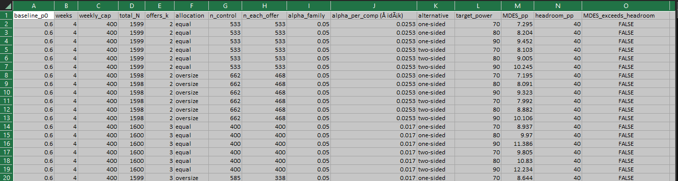
All that one has to do is to filter the columns whose values they know and read the values for the columns whose values they might be interested in. If one doesn’t find those values, you might want to look for two values closest to them (+/- both) and extrapolate the values desired! If that doesn’t work, perhaps run the code for the values that you know to find out the values desired.

Let me know if it is something that you found helpful!