Cracking Time Complexity: How to Analyze Recursive & Layered Problems
Analyzing time complexity can be tricky, especially for recursive or multi-layered problems — and it’s a critical skill in technical…
Cracking Time Complexity: How to Analyze Recursive & Layered Problems
Analyzing time complexity can be tricky, especially for recursive or multi-layered problems — and it’s a critical skill in technical interviews. In this post, we’ll break down approaches to master time complexity analysis: from recurrence relations and the master theorem to recognizing common patterns. You’ll also learn when (and why) to choose between data structures like heaps, and how to avoid the common mistakes that trip up interview candidates.
Definition of Constant Time Complexity O(1)
Before we delve into the world of time complexity, let us understand what “constant” means. A constant operation has a time complexity of O(1) and can be ignored in your complexity calculations. Often, you have been told to ask about input size — this is precisely the reason why. If your input size is always fixed and doesn’t depend on the value of n, you are dealing with constants.
🔥 Top Tech Jobs Are Hiring NOW — Don’t Miss Out.
🚀 Multiple Roles Available 👉 Apply & Secure Your Job
Key Insight: If your input size is bounded by a fixed limit that doesn’t scale with the problem, it contributes O(1) to your complexity.
Time Complexity Example
Consider a scenario where you always process a fixed number of characters (say the English alphabet: a-z). Even if you iterate through all 26 letters, this is still O(1) because the number 26 is a constant independent of n.
// O(1) time - fixed character set
public int countUniqueLetters(String word) {
    // Assuming input contains only lowercase English letters (a-z)
    boolean[] seen = new boolean[26];  // Fixed size, always 26
    for (char c : word.toCharArray()) {
        seen[c - 'a'] = true;  // O(1) operation per character
    }
    int count = 0;
    for (boolean b : seen) {
        if (b) count++;
    }
    return count;  // Returns at most 26, so O(1) space
}
Space Complexity Example
The same principle applies to space. If you use a set or map to store a fixed number of characters (say 26 letters), the space complexity is O(1) — not O(n) — because the space doesn’t scale with the problem size.
// O(1) space - bounded character set
public boolean isAnagram(String s1, String s2) {
    if (s1.length() != s2.length()) return false;

    Map<Character, Integer> charCount = new HashMap<>();
    for (char c : s1.toCharArray()) {
        charCount.put(c, charCount.getOrDefault(c, 0) + 1);
    }
    // charCount will have at most 26 entries, so O(1) space

    for (char c : s2.toCharArray()) {
        if (!charCount.containsKey(c)) return false;
        charCount.put(c, charCount.get(c) - 1);
    }
    return true;
}
Why This Matters in Interviews
This distinction can save you in technical interviews. If you can prove your space complexity is O(1) because the input size is bounded by a constant, you’ve just optimized a solution that might otherwise look inefficient. Always clarify the input constraints — it can turn what looks like an O(n) solution into an O(1) one.
Linear Time Complexity O(n)
Let us start simple. If you are given n values and you need to look at all n values to make a decision, your time complexity is at least O(n). The time complexity may be higher depending on how that logic depends on other elements. For this specific part, assume you are running a for/while loop and iterating over all elements.
// O(n) example - finding the maximum value
public int findMax(int[] arr) {
    int maxVal = Integer.MIN_VALUE;
    for (int num : arr) {  // O(n) iterations
        maxVal = Math.max(maxVal, num);  // O(1) work per iteration
    }
    return maxVal;
}
Important: The work being done in every loop iteration must be O(1) (constant time) with no dependency on the size of n. This is a common mistake in interviews — many candidates accidentally introduce hidden complexities inside their loops.However, one very important thing to keep in mind is that the work being done in every loop should be O(1) (or constant) and has no dependency on the size of n.
Quadratic Time Complexity O(n²)
If you take the same loop from above and perform work that depends on the size of n in every iteration, your time complexity changes from O(n) to O(n²). This is because every iteration now involves O(n) amount of work. Common culprits include nested loops or operations that scale with the input size.
The math: O(n) iterations × O(n) work per iteration = O(n²)
// O(n²) example - detecting duplicates (brute force approach)
public boolean hasDuplicates(int[] arr) {
    for (int i = 0; i < arr.length; i++) {  // O(n) outer loop
        for (int j = i + 1; j < arr.length; j++) {  // O(n) inner loop
            if (arr[i] == arr[j]) {  // O(1) comparison
                return true;
            }
        }
    }
    return false;
}
Why This Matters in Interviews: Confusing O(n) with O(n²) can cost you the job. A brute-force O(n²) solution might pass small test cases, but fail on larger inputs — and interviewers will always ask if you can optimize it. This is your cue that a better approach exists.
Logarithmic Time Complexity O(logn)
Logarithmic time complexity is the best you can have after O(1). It occurs when you repeatedly divide the problem size in half, discarding one half with each iteration. The base of the logarithm is typically 2, meaning the problem is divided into half at each step.
Building Intuition: The Halving Process
Imagine you start with a problem of size n and keep halving it until you reach size 1:
Iteration 0: n
Iteration 1: n/2
Iteration 2: n/4
Iteration 3: n/8
...
Iteration k: 1
How many iterations (k) does it take to go from n to 1?
If n/2^k = 1, then 2^k = n, so k = log₂(n)
That’s where O(log n) comes from!
Understanding Using Masters Theorem
For every iteration we are halving the input and doing some constant operation:
T(n) = T(n/2) + c

T(n) = T(n/2) + c
T(n/2) = T(n/4) + c
T(n/4) = T(n/8) + c
T(1) = 1

Summing up the operations:

Level 0: c operations
Level 1: c operations
Level 2: c operations
...
Level k: c operations

Total = k × c, where k is the number of levels = log₂(n)
Therefore: T(n) = O(log n)
Concrete Example: Binary Search
// O(log n) - Binary Search on a sorted array
public int binarySearch(int[] arr, int target) {
    int left = 0, right = arr.length - 1;

    while (left <= right) {
        int mid = left + (right - left) / 2;  // O(1)

        if (arr[mid] == target) {
            return mid;
        } else if (arr[mid] < target) {
            left = mid + 1;  // Eliminate left half
        } else {
            right = mid - 1;  // Eliminate right half
        }
    }
    return -1;
}
Each iteration eliminates half of the remaining elements, so with n elements, you need log₂(n) comparisons
Here's how O(log n) manifests in a balanced binary search tree:

                    50                 <- Level 0 (1 node)
                   /  \
                 30    70              <- Level 1 (2 nodes)
                / \    / \
              20  40  60  80           <- Level 2 (4 nodes)
             / \ / \ / \ / \
            10 25...            <- Level 3 (8 nodes)

For n = 8 elements:
Height = log₂(8) = 3 levels

To find any element: max 3 comparisons
Other O(log n) Scenarios
// O(log n) - Balanced BST insertion
public void insertBST(TreeNode root, int value) {
    // Each insertion traverses at most log(n) levels
    // because the tree is balanced
}

// O(log n) - Power calculation using divide-and-conquer
public double power(double x, int n) {
    if (n == 0) return 1.0;

    double half = power(x, n / 2);  // Divide problem by 2

    if (n % 2 == 0) {
        return half * half;
    } else {
        return half * half * x;
    }
}
Note that if you are making the problem size 1/3rd of what it is in every level then your time complexity is still logarithmic but the base changes to 3. It doesn’t matter in terms of time complexity but worth noting it down.
Why This Matters in Interviews
O(log n) is a massive optimization. Converting a brute-force O(n) solution to O(log n) is one of the best improvements you can make. Interviewers will often hint at this:
- “The array is sorted” → Think binary search (O(log n))
- “Use a balanced tree structure” → Implies O(log n) operations
- “Divide and conquer” → Often leads to O(log n)
Loglinear Time Complexity O(n log n)
We learned that picking one element from a sorted array is O(log n). If you have an array of size n and we have to do it for all n elements to find its right position (using merge sort), we are looking at O(n log n) time complexity. No wonder popular and most efficient sorting techniques use O(n log n) time complexity. If your code requires you to sort an array of size n, you should consider this time complexity into your calculation.
Note that if you have an array or a collection of size n, where you sort it directly, or you use a data structure such as TreeSet or a Priority Queue, you are looking at the same time complexity of O(n log n). However, it is where things get interesting with Priority Queue.
Priority Queue (Heap) and Loglinear Time Complexity
Let us clarify the time complexity with min and max heaps before we get deeper into complex use cases:
Inserting and removing the top element from a Priority Queue of size n is O(log n). However, if you need to search for an element or update an element after searching it — you are looking at a time complexity of O(n). Therefore, never use Priority Queue for lookup or update operations. If you must, use another data structure (such as HashMap) for quick lookup and update. This is precisely what Redis Sorted Set does (it uses SkipList instead of priority queue but the idea is the same).
Peeking the top element from the heap is O(1). This is what makes max and min heaps very attractive for efficiently finding and extracting top or bottom k elements. Since we are on this topic, I want to clarify the selection of the right data structure for finding top K. A common point of confusion for finding the top k highest numbers is to use a max heap. Let us see why it isn’t the best data structure.
Max Heap vs Min Heap for Top K
We store k elements in the heap so storing the k elements in the max heap when we have n elements will be O(n log k). Why? It is because our heap is sized to k and each insert will be O(log k) and we iterate over all n elements to arrive at O(n log k).
When we insert elements into a max heap, we want to insert only when the incoming element is higher than our current values. To know which element our current element can replace, we need to find the minimum of the k elements currently in the heap — which requires searching the heap, taking O(k) time. Then we remove it and insert the new element with a time complexity of O(log k). So the time complexity per element becomes O(k + log k) = O(k), and for all n elements it becomes O(n k), which is much higher.
Instead, if we use a min heap for the same scenario, we will store the k largest elements in our heap. Again, like max heap, storing k elements in min heap is still O(n log k). Where min heap shines is: when we get a new element, we can peek at the current minimum (O(1)) and immediately compare it. If the current minimum is smaller than the incoming element, we remove the min and insert the new element with a time complexity of O(log k). So overall time complexity for the min heap is O(n log k).
TreeSet vs Priority Queue
When you are dealing with a collection of size n and need to search for a specific element, TreeSet has an additional advantage compared to Priority Queue. The TreeSet wins for the lookup cost. The time complexity to find an element in TreeSet is O(log n) but in Priority Queue it is O(n) since it is not fully sorted.
Priority Queue is the best choice when you can choose a size k out of n that you can use for sorting and building results. If you’re still working on data size of n, you should consider other aspects of your requirement prior to selecting the data structure.
Exponential time complexity (O(k^n))
An exponential time complexity is very typical of recursion that does work at every recursive level. For example, if we perform a DFS and in every method call we are traversing 4 paths (one for each direction), and our traversal is constrained by some limit (such as searching for a word with length l), we would be doing 4 branches at every level. Since we would be doing this for every level until we reach length l, our time complexity for a single DFS is O(4^l).
However, when we iterate through all cells in a grid (M × N), and from each cell we perform this DFS, our overall time complexity becomes O(M × N × 4^l).
Understanding with an Example
Consider a word search problem where you need to find a word in a 2D grid:
Outer loop: O(M × N)
  - Iterate through all cells as starting points

DFS from each cell: O(4^L)
  - At each level, we have 4 branches (up, down, left, right)
  - We go L levels deep (word length)
  - Total nodes explored: 4^L
Total: O(M × N × 4^L)
Important Note on Visited Sets
You might think: “If I use a visited set to prevent revisiting cells, won’t the complexity reduce to O(M × N)?”
The answer depends on how you use the visited set:
- Local visited set (backtracking): If the visited set is local to each DFS path and you unmark cells as you backtrack, different paths can still revisit the same cell. In this case, the complexity remains O(M × N × 4^L).
- Global visited set: If you prevent any cell from being visited across all DFS calls, you visit each cell at most once. In this case, the complexity reduces to O(M × N).
In most word search problems like Leetcode 79, the visited set is local to each DFS path (backtracking), so the O(M × N × 4^L) complexity applies.
Practice Problems
Problem 1: Simple Loop
for i = 0 to n:
    print i
Problem 2: Nested Loops
for i = 0 to n:
    for j = 0 to n:
        arr[i][j] = i + j
Problem 3: Binary Search
function binarySearch(arr, target):
    left = 0
    right = arr.length - 1
    while left <= right:
        mid = (left + right) / 2
        if arr[mid] == target:
            return mid
        else if arr[mid] < target:
            left = mid + 1
        else:
            right = mid - 1
    return -1
Problem 4: Merge Sort
function mergeSort(arr, left, right):
    if left < right:
        mid = (left + right) / 2
        mergeSort(arr, left, mid)
        mergeSort(arr, mid + 1, right)
        merge(arr, left, mid, right)  // O(n) operation
Problem 5: Finding Top K Elements with Min Heap
function findTopK(arr, k):
    minHeap = new PriorityQueue(k)
    for each element in arr:  // n iterations
        if minHeap.size() < k:
            minHeap.insert(element)  // O(log k)
        else if element > minHeap.peek():
            minHeap.remove()  // O(log k)
            minHeap.insert(element)  // O(log k)
    return minHeap
Problem 6: Checking for Duplicates (Brute Force)
function hasDuplicates(arr):
    for i = 0 to arr.length:
        for j = i + 1 to arr.length:
            if arr[i] == arr[j]:
                return true
    return false
Problem 7: Permutations (Recursive)
function generatePermutations(str, result):
    if str.length == 0:
        result.add("")
        return
    for i = 0 to str.length:
        char = str[i]
        remaining = str without str[i]
        generatePermutations(remaining, result)
Problem 8: Balanced Binary Search Tree — Search
function searchBST(root, target):
    if root == null:
        return false
    if root.value == target:
        return true
    else if root.value > target:
        return searchBST(root.left, target)
    else:
        return searchBST(root.right, target)
Problem 9: String Concatenation in Loop
function concatenateStrings(strings):
    result = ""
    for each str in strings:  // n strings
        result = result + str  // concatenation
    return result
Problem 10: Processing Elements with Sorted Order
function processWithTreeSet(arr):
    treeSet = new TreeSet()
    for each element in arr:  // n elements
        treeSet.insert(element)  // insertion into sorted structure
    for each element in treeSet:
        process(element)  // O(1) operation
    return result
Conclusion: Mastering Time Complexity Analysis
Time complexity analysis isn’t just theoretical — it’s a practical skill that separates strong engineers from average ones. Throughout this guide, we’ve explored how to think about complexity: from recognizing constant operations to understanding exponential recursion. But knowledge alone won’t carry you through an interview.
During technical interviews, several patterns will emerge repeatedly. First, always clarify input constraints with your interviewer — this seemingly simple step can transform what looks like an O(n) solution into an O(1) one. Second, watch for halving patterns in the problem. When you see sorting, binary search, or divide-and-conquer approaches, O(log n) is likely in play. Third, be wary of nested structures. Multiple loops often hint at O(n²) or worse, and interviewers will push you to optimize.
You’ll also encounter situations where data structure selection matters. Remember that min heaps are your ally for finding top K elements with O(n log k) complexity, not max heaps. And when analyzing recursive problems that feel tricky, don’t hesitate to write out the Master’s Theorem — it’s a reliable way to break down complexity that might otherwise feel overwhelming.
The real mastery comes from practice. Solve the 10 practice problems we’ve included, then move on to real Leetcode problems and interview questions. Analyze solutions not just for correctness, but for their time and space complexity. Soon, you’ll develop an intuition where complexity analysis becomes second nature — you’ll glance at code and immediately know its complexity profile.
Time complexity is one of those skills that, once internalized, stays with you throughout your engineering career. It influences architecture decisions, helps you spot performance bottlenecks, and earns you respect in code reviews. Start practicing today, and by the time your interview rolls around, you’ll be ready.
Good luck with your interviews!
메타데이터
- post_id
- f3ba5c1ccc87
- slug
- cracking-time-complexity-how-to-analyze-recursive-layered-problems-f3ba5c1ccc87
- url
- https://medium.com/@sinha.k/cracking-time-complexity-how-to-analyze-recursive-layered-problems-f3ba5c1ccc87
- canonical_url
- https://medium.com/@sinha.k/cracking-time-complexity-how-to-analyze-recursive-layered-problems-f3ba5c1ccc87
- author_url
- https://medium.com/@sinha.k
- status
- ok
- fetched_at
- 2026-06-15 22:55:51