Getting Started with AstraeaDB in R: A Graph + Vector Database in Minutes

Build a small movie knowledge graph, traverse it, and query it, all from R.

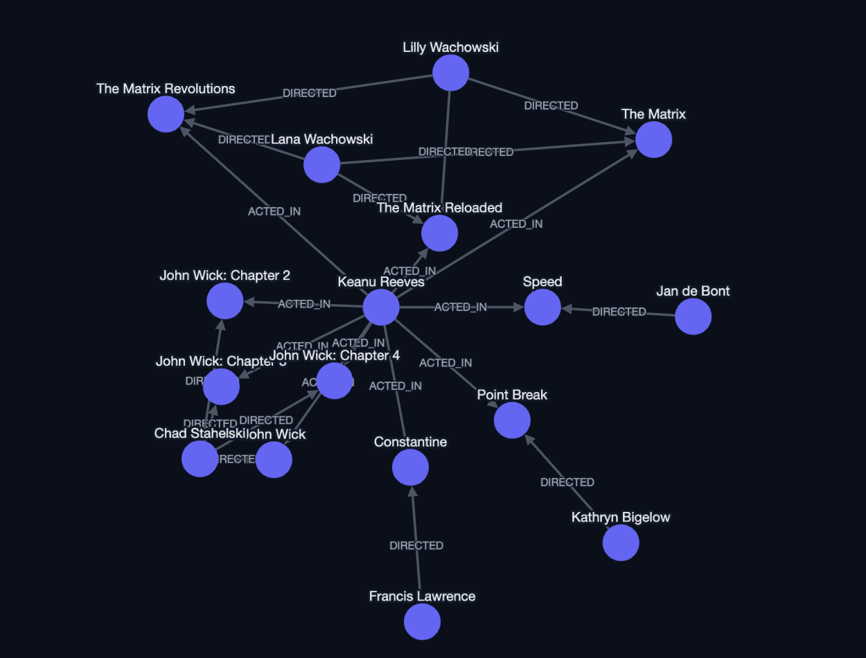
Example Dashboard in Shiny/R for AstraeaDB

Most databases make you choose. You keep one kind of store for the relationships between things, a second kind for searching by meaning, and then you write a lot of extra code to keep the two in sync. AstraeaDB removes that tradeoff. It is a graph database, written in the Rust programming language and designed for artificial-intelligence (AI) work, that stores your data in two complementary ways at the same time. First, it keeps a graph: labeled nodes and the edges (the relationships) between them, where both nodes and edges can carry properties such as a title or a name. Second, it keeps an index over embeddings, which are lists of numbers that capture the meaning of a piece of text, so it can quickly find items whose meanings are similar (a task often called semantic search). Because both live in the same store, following relationships and searching by meaning work side by side. AstraeaDB calls this combined model a Vector-Property Graph. In this first post we will stay on the graph side: install the server, connect from R, build a tiny movie knowledge graph, and read it back with a few traversals and a query. Vectors are the subject of post 2.

Installing and running the server

The R client is a thin layer of code that talks to a running AstraeaDB server. The two communicate over a local network connection at the address 127.0.0.1:7687, where 127.0.0.1 simply means “this same computer.” They exchange messages in JSON, a common plain-text format for structured data, though you never have to handle that format yourself. So the first step is getting the server up. It ships as a program you install with cargo, the build tool that comes with Rust. If you do not already have a Rust toolchain, get one from rustup.rs first.

Building the server also relies on Protocol Buffers, a data format from Google, so on a fresh Linux machine you first need a few system packages. On Debian or Ubuntu, one command installs all of them:

sudo apt-get install -y protobuf-compiler libprotobuf-dev pkg-config libssl-dev build-essential

On macOS with Homebrew, the equivalent is brew install protobuf.

# Installs the `astraeadb` binary (compiles from source; takes a few minutes)
cargo install --git https://github.com/AstraeaDB/AstraeaDB-Official.git astraea-cli

# Start the server (JSON/TCP on 127.0.0.1:7687, data persisted to disk)
astraeadb serve

Leave that terminal running, because it is now your database. A few other subcommands are worth knowing. astraeadb status runs a quick health check. astraeadb shell opens an interactive prompt where you type commands and see results right away. astraeadb serve --port 7700 overrides the default port when 7687 is already taken. Everything below runs in a second terminal (or an R session) while the server keeps running in the first.

Installing the R client and connecting

Update as of 8/21/2026: The official package has been released on CRAN

̶T̶h̶e̶ ̶c̶l̶i̶e̶n̶t̶ ̶h̶a̶s̶ ̶b̶e̶e̶n̶ ̶s̶u̶b̶m̶i̶t̶t̶e̶d̶ ̶t̶o̶ ̶C̶R̶A̶N̶,̶ ̶t̶h̶e̶ ̶C̶o̶m̶p̶r̶e̶h̶e̶n̶s̶i̶v̶e̶ ̶R̶ ̶A̶r̶c̶h̶i̶v̶e̶ ̶N̶e̶t̶w̶o̶r̶k̶,̶ ̶w̶h̶i̶c̶h̶ ̶i̶s̶ ̶t̶h̶e̶ ̶o̶f̶f̶i̶c̶i̶a̶l̶ ̶p̶l̶a̶c̶e̶ ̶R̶ ̶d̶o̶w̶n̶l̶o̶a̶d̶s̶ ̶p̶a̶c̶k̶a̶g̶e̶s̶ ̶f̶r̶o̶m̶.̶ ̶T̶h̶e̶ ̶p̶a̶c̶k̶a̶g̶e̶ ̶i̶s̶ ̶c̶u̶r̶r̶e̶n̶t̶l̶y̶ ̶a̶w̶a̶i̶t̶i̶n̶g̶ ̶m̶a̶n̶u̶a̶l̶ ̶r̶e̶v̶i̶e̶w̶ ̶(̶e̶x̶p̶e̶c̶t̶e̶d̶ ̶w̶i̶t̶h̶i̶n̶ ̶t̶h̶e̶ ̶n̶e̶x̶t̶ ̶f̶e̶w̶ ̶d̶a̶y̶s̶)̶.̶ Once it appears on CRAN, installing it is the usual one-liner:

install.packages("AstraeaDB")

If it has not reached your CRAN mirror yet, you can install the development version straight from GitHub instead. It is the same package with the same functions:

# install.packages("remotes")
remotes::install_github("AstraeaDB/R-AstraeaDB")

Now you can connect. The package gives you a client object, and you call its functions (its methods) using the $ sign, as in client$create_node(...). Before you start, it is worth checking that the server is actually reachable:

library(AstraeaDB)

if (!astraea_server_available()) {
  stop("Start the server first: run `astraeadb serve` in a terminal.")
}

client <- astraea_connect()   # defaults: host = "127.0.0.1", port = 7687L

That client object is what we will use for everything else. When you are finished, call client$disconnect() to close the connection cleanly.

Building a movie knowledge graph

A knowledge graph is simply a set of things (called nodes) connected by relationships (called edges), where both the things and the relationships can carry properties. We will model a handful of movies, the people who made them, and a couple of genres. Every node has one or more labels, which describe its type, along with a list of properties. The create_node function returns the node’s integer ID, and we store that ID in a variable so we can attach edges to it later.

# Movies: labels + properties (we'll add plot embeddings in post 2)
matrix     <- client$create_node(c("Movie"), list(title = "The Matrix", year = 1999L,
                                   plot = "A hacker discovers reality is a simulation."))
reloaded   <- client$create_node(c("Movie"), list(title = "The Matrix Reloaded", year = 2003L,
                                   plot = "Neo takes the fight to the machines."))
wick       <- client$create_node(c("Movie"), list(title = "John Wick", year = 2014L,
                                   plot = "A retired hitman is pulled back for revenge."))
inception  <- client$create_node(c("Movie"), list(title = "Inception", year = 2010L,
                                   plot = "A thief steals secrets from dreams."))
darkknight <- client$create_node(c("Movie"), list(title = "The Dark Knight", year = 2008L,
                                   plot = "Batman confronts the Joker."))

# People: actors and directors
keanu <- client$create_node(c("Person"), list(name = "Keanu Reeves"))
lana  <- client$create_node(c("Person"), list(name = "Lana Wachowski"))
nolan <- client$create_node(c("Person"), list(name = "Christopher Nolan"))
leo   <- client$create_node(c("Person"), list(name = "Leonardo DiCaprio"))
bale  <- client$create_node(c("Person"), list(name = "Christian Bale"))

# Genres
scifi  <- client$create_node(c("Genre"), list(name = "Sci-Fi"))
action <- client$create_node(c("Genre"), list(name = "Action"))

Now we create the relationships. Edges are directed, meaning each one points from a source node to a target node, and every edge has a type. The create_edge(source, target, edge_type) function returns an edge ID, which we do not need to keep here. We will use three edge types: ACTED_IN and DIRECTED run from a Person to a Movie, and IN_GENRE runs from a Movie to a Genre.

# Who acted in what
client$create_edge(keanu, matrix,     "ACTED_IN")
client$create_edge(keanu, reloaded,   "ACTED_IN")
client$create_edge(keanu, wick,       "ACTED_IN")
client$create_edge(leo,   inception,  "ACTED_IN")
client$create_edge(bale,  darkknight, "ACTED_IN")

# Who directed what
client$create_edge(lana,  matrix,     "DIRECTED")
client$create_edge(nolan, inception,  "DIRECTED")
client$create_edge(nolan, darkknight, "DIRECTED")

# Genres
client$create_edge(matrix,     scifi,  "IN_GENRE")
client$create_edge(matrix,     action, "IN_GENRE")
client$create_edge(reloaded,   scifi,  "IN_GENRE")
client$create_edge(wick,       action, "IN_GENRE")
client$create_edge(inception,  scifi,  "IN_GENRE")
client$create_edge(darkknight, action, "IN_GENRE")

That gives us 12 nodes and 14 edges, a small but complete graph.

Reading it back

Let us confirm what we stored. The get_node function returns a list with the node’s labels and its properties:

client$get_node(matrix)
# $labels     -> "Movie"
# $properties -> list(title = "The Matrix", year = 1999, plot = "...")

The real strength of a graph is that you can ask about connections. The neighbors function walks the edges leading out of or into a node. Direction matters here. "outgoing" follows edges where the node is the source, "incoming" follows edges where it is the target, and "both" ignores direction. You can also filter by edge type.

# Movies Keanu acted in (follow his outgoing ACTED_IN edges)
client$neighbors(keanu, direction = "outgoing", edge_type = "ACTED_IN")

# Everyone connected TO The Matrix: its actors and director (incoming edges)
client$neighbors(matrix, direction = "incoming")

To collect every node of a given type, use find_by_label, which returns a list of node IDs:

client$find_by_label("Movie")   # the five Movie IDs

First traversals

Nearest Neighbors

A neighbor is one step away. A traversal goes further by following a chain of edges across the graph. Breadth-first search, available as bfs, fans out one level at a time and reports each node it can reach along with that node’s depth, meaning how many steps away it is. Depth-first search, available as dfs, instead follows each branch as far as it goes before backing up, and it returns node IDs. Starting from Keanu with a depth limit of 2, breadth-first search reaches his movies at depth 1 and their genres at depth 2.

client$bfs(keanu, max_depth = 2L)   # list of { node_id, depth }
client$dfs(keanu, max_depth = 2L)   # list of node IDs

The shortest_path function finds the route with the fewest steps between two nodes. Here the path from Keanu to the Sci-Fi genre runs through one of his movies:

client$shortest_path(keanu, scifi)
# Keanu Reeves --ACTED_IN--> The Matrix --IN_GENRE--> Sci-Fi
# $path   -> the node IDs along the route
# $length -> 2

The Path from Keanu Reeves to Sci-Fi

Pass weighted = TRUE to minimize the total edge weight rather than the number of steps. That option becomes useful once your edges carry meaningful weights, such as distances or costs.

One query in GQL

The traversal functions cover the most common questions, but sometimes you would rather describe the answer you want and let the database work out the steps. For that, AstraeaDB understands a graph query language, called GQL for short, whose style is similar to Cypher (a widely used language for querying graph databases). You send a query with client$query(), and it returns a result made up of columns and rows:

client$query("MATCH (m:Movie) RETURN m.title, m.year")
# columns: m.title, m.year
# rows:    "The Matrix" 1999, "Inception" 2010, "John Wick" 2014, ...

If you would rather work with tabular data, the client can hand the result back as a data frame, R’s built-in table structure, using client$results_to_dataframe(...). That makes it easy to pass the data along to the tidyverse, a popular collection of R packages for data analysis.

A health check with graph_stats

Finally, graph_stats gives you a bird’s-eye view of the whole store: the total number of nodes and edges, plus a breakdown by label. It is the quickest way to confirm that your data loaded correctly:

client$graph_stats()
# $total_nodes -> 12
# $total_edges -> 14
# $labels      -> Movie = 5, Person = 5, Genre = 2

client$disconnect()

Twelve nodes and fourteen edges, exactly what we built.

What’s next

You now have AstraeaDB running, a real if tiny knowledge graph inside it, and the core actions you need to create, read, traverse, and query that graph. So far this has all been graph work, the kind of thing a property-graph database handles well on its own.

AstraeaDB really exists for the other half of the picture. Those plot strings on each movie can be turned into embeddings, the lists of numbers that capture the meaning of text, and the same store that answers “who directed this?” can then also answer “find me movies with a similar feel.” In the next post, Vector and Hybrid Search with AstraeaDB in R, we will attach simple plot embeddings to our movies and use vector_search, hybrid_search, and searches that combine meaning with graph structure to turn this graph into a small recommender.