3D Reconstruction from Scratch, Part 1: Feature Extraction and the Search for Distinctive Points

Imagine taking a few photos of the same building from different angles. To us, it is easy to notice the same window corners, edges, and textured regions across those images. Our brain naturally picks out the important visual details.

A computer does not do that automatically. To a machine, an image is just a grid of numbers. Before it can understand depth, motion, or 3D structure, it must first learn where to look. It needs to identify points in an image that are distinctive, stable, and likely to be found again in another view.

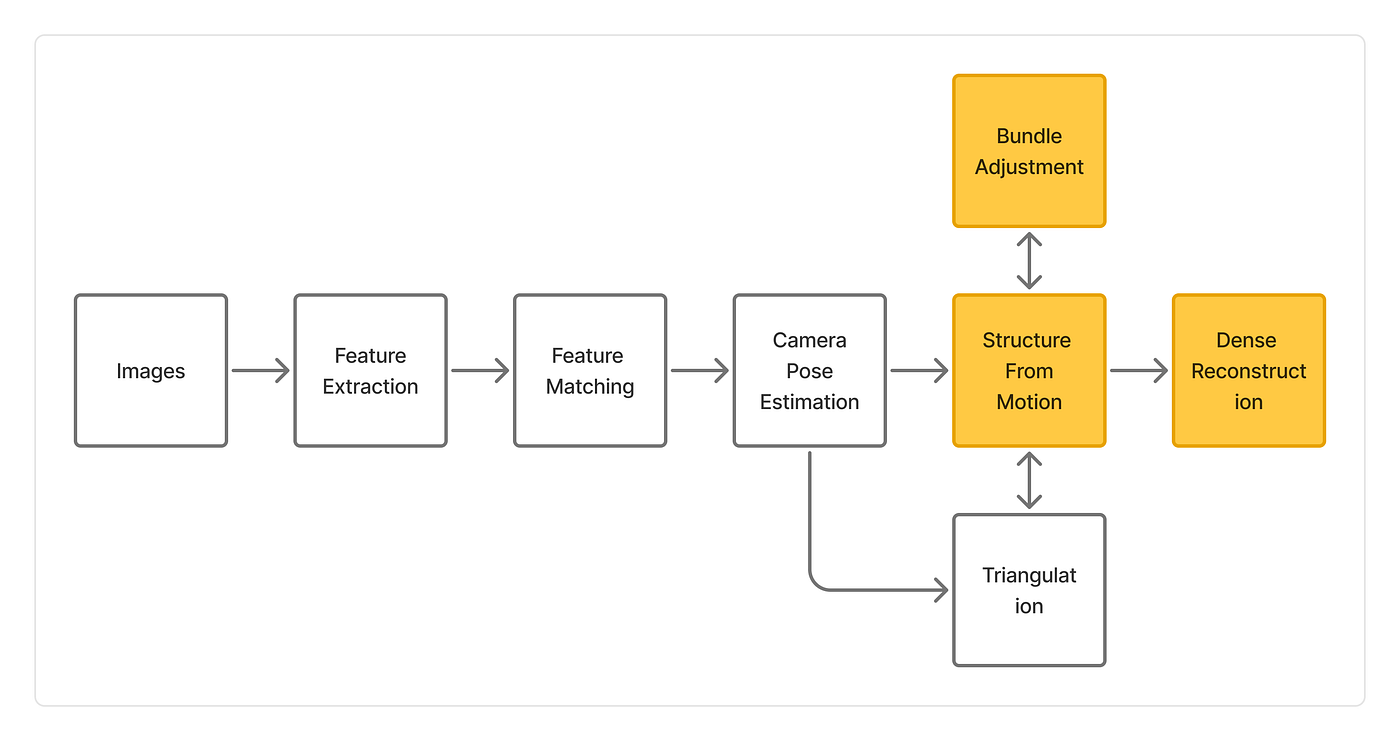
That is where feature extraction begins. It is the first real step in 3D reconstruction, and it lays the foundation for everything that comes next. Before matching points across images, before estimating camera pose, and before reconstructing 3D structure, the machine must first detect meaningful visual points and describe them in a way that makes them recognizable.

In this article, we focus entirely on that first step: feature extraction, the process of detecting keypoints, building descriptors, and understanding why methods like SIFT became so important in computer vision.

3D Reconstruction Pipeline: Feature Extraction

Introduction

At its core, 3D computer vision is about recovering the structure of the real world from images. A camera gives us only a 2D projection of a scene, yet the world itself is three-dimensional. The challenge is to bridge that gap, to infer geometry, depth, and spatial structure from flat images.

This problem appears in many important applications. In robotics, machines need to understand their surroundings to navigate and interact safely. In autonomous driving, vehicles must estimate the 3D layout of roads, obstacles, and other agents. In augmented reality, virtual objects must be placed consistently within the real world. In mapping, surveying, cultural heritage preservation, and drone-based reconstruction, image collections are turned into digital 3D models of real environments.

But none of this begins directly with 3D points. Before a machine can estimate camera motion or reconstruct structure, it must first decide what in an image is worth paying attention to. Not every pixel is informative. Large flat regions often look the same everywhere, while some locations, like corners, textured patches, and distinctive local patterns, carry much richer visual information. These are the parts of the image that are more likely to be detected again from another viewpoint.

This is where feature extraction becomes essential. Feature extraction is the process of detecting distinctive image points and representing the appearance around them in a compact and meaningful way. These points, often called keypoints, and their numerical representations, called descriptors, form the foundation for later stages of reconstruction. If these features are not stable and informative, everything that follows becomes unreliable.

In this article, we focus entirely on that first step. We will understand what makes a good feature, why some parts of an image are more useful than others, and how feature extraction is formulated both intuitively and mathematically. From there, we will dive deeply into SIFT (Scale-Invariant Feature Transform), one of the most important classical methods in computer vision, and study how it detects stable keypoints across scale, assigns orientation, and builds robust local descriptors.

Before a system can understand a scene in 3D, it must first learn to identify the image details worth remembering.

Feature Extraction

Before a computer can match points across images, it must first decide what is worth paying attention to in an image. This is the role of feature extraction.

At a high level, feature extraction is the process of finding visually distinctive parts of an image and representing them in a form that can be recognized again in another image. These distinctive parts are usually called features or keypoints.

Think about an image of a building. Not every pixel is equally useful. A large blank wall contains many pixels, but most of them look nearly identical. If you pick one pixel in the middle of that wall, it becomes very hard to find that same point in another image. On the other hand, the corner of a window, the edge where two surfaces meet, or a textured patch on the ground tends to stand out. These are the kinds of locations that are much easier to detect again from another viewpoint.

That is why 3D reconstruction does not start by using the whole image directly. It starts by finding a smaller set of points that are stable, distinctive, and repeatable.

What is a feature?

A feature is a meaningful visual pattern in an image that can help identify the same scene content across different views. In practice, when we talk about local feature extraction, we usually mean two things:

• a keypoint, which tells us where in the image something interesting is located
• a descriptor, which tells us what the local appearance around that point looks like

So a feature is not just a point. It is really a combination of:

1. a location in the image, and
2. a numerical description of the neighborhood around that location

This distinction is important.

If we only detect keypoints, we know where interesting points are, but we do not yet know how to compare them across images. If we only have descriptors without stable keypoints, then the locations themselves may not be reliable. A useful feature extraction pipeline must therefore answer both questions:

• Where are the important points?
• How can I describe them so I can recognize them later?

What is a keypoint?

A keypoint is a point in the image that stands out from its surroundings. It is a location that is likely to be detected again even if the image is resized, rotated, viewed from a slightly different angle, or affected by some lighting changes.

Good keypoints often occur at:

• corners
• blobs
• junctions
• textured regions
• highly distinctive local structures

They usually do not occur in:

• flat, uniform regions
• repetitive, ambiguous regions
• weak, noisy areas with little local structure

For example, imagine three kinds of image regions:

• On a flat wall, all nearby pixels look almost the same. There is no strong visual clue to lock onto.
• Along a simple edge, there is some intensity change, but motion along the edge direction is ambiguous.
• At a corner, intensity changes strongly in more than one direction, making that point much easier to localize and rediscover.

This is one reason corners are often such useful keypoints.

What is a descriptor?

Once a keypoint is found, we still need to describe the local image content around it. That description is called a descriptor.

A descriptor is usually a vector of numbers that captures the appearance of the neighborhood around the keypoint compactly and robustly. The idea is that if two keypoints in different images come from the same real-world point, then their descriptors should be similar.

So while the keypoint says:

“Look here.”

The descriptor says:

“This is what the neighborhood around this point looks like.”

For example, a descriptor may encode:

• local gradient directions
• gradient magnitudes
• intensity patterns
• orientation structure
• texture information

In SIFT, which we will study in detail next, each keypoint is assigned a 128-dimensional descriptor vector built from local gradient histograms.

Why is feature extraction necessary?

At first glance, you might ask: why not simply compare whole images pixel by pixel?

The problem is that real images change a lot across viewpoints. The same scene captured from two positions can differ because of:

• camera motion
• scale change
• rotation
• viewpoint change
• illumination variation
• partial occlusion
• noise
• blur

A raw pixel at one position in image A does not usually line up directly with the same pixel position in image B. This makes direct comparison unreliable.

Feature extraction solves this by focusing only on local, distinctive structures that are more likely to survive those changes. Instead of trying to compare every pixel, we compare a much smaller set of robust image landmarks. This dramatically reduces the problem complexity and makes matching much more meaningful.

The mathematical view of an image

To understand feature extraction more clearly, it helps to think of an image mathematically.

A grayscale image can be represented as a function:

where:

• x and y represent image coordinates
• I(x,y) gives the intensity value at that location

In a color image, we may have multiple channels, but the main idea remains the same.

Feature extraction is essentially about studying how this intensity function behaves locally. We are interested in points where the image structure changes in a meaningful way.

For example:

• in a flat region, I(x,y) changes very little
• along an edge, I(x,y) changes strongly in one direction
• at a corner or textured point, I(x,y) changes in multiple directions

Those local variations are what make some points informative and others useless.

What makes a good feature?

Not every detected point is useful. A good feature should satisfy several properties.

1. Repeatability

A feature should be detectable again in another image of the same scene. This is one of the most important requirements. If a point is found in one image but disappears in the next, it is not useful for matching or reconstruction.

2. Distinctiveness

A feature should look sufficiently different from other points. If many locations produce almost the same descriptor, then matching becomes ambiguous. Distinctive points reduce false matches.

3. Localization accuracy

A feature should be localized precisely. In 3D reconstruction, even small errors in point position can affect pose estimation and triangulation. So features should not only be detectable, but also accurately placed.

4. Robustness to scale

The same physical point may appear larger or smaller depending on the camera distance. A good feature detector should still detect that point even if the image scale changes.

5. Robustness to rotation

If the camera rotates, the local appearance also rotates. A useful feature should still be recognized after rotation.

6. Robustness to illumination changes

Lighting conditions may differ between images. Although no handcrafted feature is perfectly invariant to lighting, a good one should tolerate moderate brightness and contrast changes.

7. Robustness to noise and blur

Real images are imperfect. Noise, compression artifacts, and motion blur can all corrupt image details. A strong feature extractor should not fail under mild distortions.

8. Computational efficiency

In practical systems, extraction should not be excessively expensive. This matters especially in robotics, SLAM, and large-scale reconstruction, where many images must be processed.

Now that we understand what feature extraction is and what makes a feature useful, we are ready to study one of the most important handcrafted local feature methods in computer vision: SIFT, or Scale-Invariant Feature Transform.

SIFT is not just a detector, nor is it just a descriptor. It is a complete pipeline for:

• finding stable keypoints across scales,
• assigning them consistent orientations,
• and describing their local appearance in a way that is robust and highly distinctive.

To understand why SIFT works so well, we need to begin with one of its central ideas: scale-space.

SIFT: Scale-Invariant Feature Transform

SIFT is one of the most influential feature extraction methods in computer vision. Introduced by David Lowe, it was designed to detect and describe local image features in a way that is robust to changes in scale, rotation, moderate illumination, and small viewpoint variations.

That is exactly why it became so important in image matching, object recognition, SLAM, and 3D reconstruction.

At a high level, SIFT does four major things:

1. It searches for stable keypoints across different image scales
2. It removes unstable or poorly localized points
3. It assigns a consistent orientation to each keypoint
4. It builds a distinctive descriptor around each keypoint

This is what makes SIFT so powerful: it is not just detecting points, it is building features that can actually be matched reliably later.

Why scale matters?

Before understanding how SIFT works, we need to understand the problem it was designed to solve.

Imagine taking two photographs of the same building:

• one from far away
• one from much closer

The same window corner appears in both images, but not at the same size. In one image, it may occupy a tiny patch. In the other, it may cover a much larger region.

If a detector only works at one fixed image scale, then it may detect the point in one image and miss it in the other. This is a serious problem, because in real-world vision, the same physical point rarely appears at the same size across all views.

So SIFT asks a deeper question:

Can we detect features in a way that is independent of the image scale at which they appear?

The idea of scale-space

A real image contains structure at many levels of detail. At a fine scale, you can see tiny textures, edges, and noise. At a coarser scale, small details disappear, and only larger structures remain.

To analyze image features properly, we should not look at the image at just one level of detail. We should look at it across many scales.

SIFT does this by creating a scale-space representation of the image.

Mathematically, the scale-space of an image is defined by convolving the image I(x,y) with a Gaussian kernel G(x,y,σ):

where:

• I(x,y) is the original image
• G(x,y,σ) is a Gaussian with scale parameter σ
• L(x,y,σ) is the smoothed image at scale σ
• • denotes convolution

The Gaussian function is:

What this means intuitively

The Gaussian blur smooths the image.

• small σ means light blur, so fine details remain visible
• large σ means stronger blur, so only coarse structures remain

By varying σ, we get multiple versions of the same image, each representing a different observation scale.

This gives us a way to ask:

At what scale is a given image structure most stable and distinctive?

That is a key idea in SIFT.

Why Gaussian smoothing?

You might ask: why use a Gaussian specifically?

The Gaussian is not chosen arbitrarily. It has several important properties:

• It smooths noise in a natural way
• It preserves coarse structure while suppressing fine detail
• It behaves well mathematically under repeated smoothing
• It provides a principled way to build scale-space

In fact, Gaussian scale-space is the standard framework for multi-scale image analysis. So when SIFT analyzes features across scale, it is really analyzing how image structures behave after repeated Gaussian smoothing.

From scale-space to keypoint detection: Now that we have multiple blurred versions of the image, we need a way to detect interesting points across those scales.

SIFT does not directly search for maxima or minima in the blurred images themselves. Instead, it computes the Difference of Gaussians, usually written as DoG. This is one of the core ideas in the whole method.

Step 1: Difference of Gaussians (DoG)

The Difference of Gaussians is computed by subtracting two nearby scale levels:

where:

• L(x,y,σ) is the Gaussian-smoothed image at scale σ
• L(x,y,kσ) is the smoothed image at a slightly larger scale
• k is a constant multiplicative factor between adjacent scales

So the DoG image measures how the image changes between two nearby blur levels.

Intuition behind DoG

If a structure is stable and important at a certain scale, it will stand out when comparing nearby scales. The DoG emphasizes regions where intensity patterns change significantly with scale. These are often blob-like or distinctive local structures. You can think of DoG as highlighting image structures that are “special” relative to both:

• their local spatial neighborhood, and
• their neighboring scales

That is why it is such a good tool for keypoint detection.

Building the DoG pyramid

To apply this across the full image, SIFT builds a pyramid structure called Octave.

An octave is a group of images covering a range of scales. After finishing one octave, the image is downsampled, usually by a factor of 2, to begin the next octave. Inside each octave, the image is repeatedly blurred using increasing values of σ. Adjacent blurred images are then subtracted to produce DoG images.

So the process looks like this:

• start with an image
• create several Gaussian-smoothed versions at increasing scales
• subtract neighboring blurred images
• Obtain a stack of DoG images
• Repeat at lower image resolution for the next octave

This allows SIFT to search for features both:

• at fine detail levels
• and at larger image structures

Detecting extrema in scale-space

Now comes the actual keypoint detection step. SIFT looks for local extrema in the DoG pyramid. A candidate keypoint is a point that is either:

• greater than all of its neighbors, or
• less than all of its neighbors

But here is the important part: The comparison is not only in the 2D image plane. It is also across scales. Each candidate point is compared against:

• 8 neighbors in the current DoG image
• 9 neighbors in the scale above
• 9 neighbors in the scale below

That gives a total of 26 neighbors.

If the point is a local maximum or minimum among all of them, it is considered a candidate keypoint.

Why compare across scales too?

Because we do not just want points that stand out spatially. We want points that stand out at a particular scale. A keypoint should be distinctive not only in its local image region, but also in how it behaves across levels of blur. This is what gives SIFT its scale invariance.

Step 2: Keypoint localization

After detecting extrema in the DoG pyramid, SIFT refines the location of each candidate keypoint. This step is important because the initial extrema are found on a discrete pixel grid and at discrete sampled scales. But the true extremum may lie between those samples.

So SIFT fits a local model around each candidate to estimate a more accurate location in:

• x
• y
• scale σ

This improves localization accuracy and removes unstable points. To refine the extremum, SIFT uses a Taylor expansion of the DoG function around the candidate point:

where x=(x,y,σ)T.

By solving for the offset that gives the extremum, SIFT estimates the subpixel and subscale location of the keypoint. You do not need to think of this as “complicated calculus first.” Intuitively, SIFT is just fitting a smooth local surface around the detected point and asking:

Where is the true peak or valley of this surface?

That gives a more accurate keypoint than simply taking the nearest sampled pixel.

Rejecting low-contrast keypoints

Some extrema are very weak. They may come from noise or insignificant image fluctuations. Such points are not reliable for matching.

So SIFT checks the DoG value at the refined location. If the response magnitude is too small, the point is discarded.

Intuition: A strong keypoint should produce a noticeable response in the DoG image. A weak response suggests the point is not stable or distinctive enough.

This helps remove noisy detections and low-information regions.

Rejecting edge responses

This is another very important filtering step. Some points may produce strong DoG responses but still be bad keypoints. This often happens along edges.

Why are edges problematic?

Because a point on a long edge may be well localized across the edge direction but poorly localized along the edge itself. That makes matching unstable.SIFT detects such cases using the Hessian matrix, which captures second-order local image structure. The Hessian has the form:

where:

• Dxx and Dyy​ are second derivatives
• Dxy​ is the mixed derivative

Intuition of the Hessian test

The eigenvalues of this matrix describe curvature in different directions.

• If both curvatures are strong and balanced, the point is likely corner-like or blob-like
• If one curvature is much larger than the other, the point is likely edge-like

SIFT avoids explicit eigenvalue computation by using a ratio test based on the trace and determinant of the Hessian. If the ratio of principal curvatures is too high, the point is rejected.

Why this matters: This step removes unstable edge points and keeps only those keypointst hat are better localized in two directions. That makes the final feature set much more reliable.

Step 3: Orientation assignment

Up to this point, SIFT has identified stable keypoints and their characteristic scales. But there is still another major challenge:

What if the same local patch appears rotated in another image?

To handle this, SIFT assigns a consistent orientation to each keypoint. This is what gives it rotation invariance. Around each keypoint, SIFT looks at a local neighborhood in the Gaussian-smoothed image at the keypoint’s scale. For each nearby pixel, it computes the gradient magnitude and orientation:

So for each pixel in the neighborhood, we know:

• how strong the local intensity change is
• which direction that change point towards

These gradient orientations are then accumulated into a histogram, usually with 36 bins covering 360 degrees.

Why use a histogram?

Because we do not want one single noisy gradient to dominate. We want the dominant orientation pattern in the neighborhood. The peak of the histogram gives the main orientation of the keypoint. That orientation is then assigned to the keypoint.

Multiple orientations

If there are other strong peaks close to the main one, SIFT may create multiple keypoints at the same location and scale but with different orientations. This helps when the local image structure has multiple meaningful directions

Why orientation assignment work?

Suppose the image rotates. Then the local gradients rotate too. But since SIFT estimates the dominant local orientation and aligns the descriptor relative to it, the descriptor can remain comparable across rotated views. In other words, instead of describing the patch in the original image coordinate frame, SIFT describes it in the keypoint’s own local orientation frame. That is the core reason for rotation invariance.

Step 4: Descriptor construction

Now we come to the final stage of SIFT: building the descriptor. This is where the keypoint becomes matchable.

Once a keypoint has:

• a location
• a scale
• an orientation

SIFT extracts a local patch around it and describes the gradient structure inside that patch in a robust numerical form.

The descriptor should be:

• distinctive enough to separate one point from another
• robust enough to tolerate small shifts, noise, and illumination changes

SIFT achieves this by using local gradient histograms.

How the SIFT descriptor is built

A neighborhood around the keypoint is taken, typically a 16×16 window at the appropriate scale. This window is divided into a 4×4 grid of smaller cells.

For each cell:

• gradient magnitudes and orientations are computed
• An 8-bin orientation histogram is formed

So we have:

• 4×4=16 cells
• 8 orientation bins per cell

Therefore, the final descriptor has:v 16×8=128 dimensions.

That is why SIFT descriptors are 128-dimensional vectors.

Why is this design so effective

This representation captures:

• where gradient patterns occur approximately
• what orientations dominate local
• enough spatial layout to be distinctive
• enough aggregation to be robust

It does not try to memorize exact pixel intensities. Instead, it captures local structure in a softer, more stable way.

Why SIFT is robust

At this point, we can see why SIFT became so successful.

It achieves robustness through several carefully designed stages:

• Scale-space extrema detection gives scale invariance
• The orientation assignment gives rotation invariance
• A gradient-based descriptor provides local distinctiveness
• Descriptor normalization improves illumination robustness
• Contrast and edge filtering remove unstable points

SIFT is strong not because of one trick, but because every stage is designed to support stable matching.

For this part of the project, I worked with the ETH3D dataset, using the training_undistorted playground scene as the starting point for feature extraction. Since this article focuses entirely on the first step of the reconstruction pipeline, the goal here is not yet to recover camera motion or build 3D points, but simply to teach the system how to identify visually meaningful locations in an image. To do that, I use SIFT to detect distinctive keypoints and compute descriptors for each image in the scene. The script reads the images one by one, converts them to grayscale, extracts up to 100,000 keypoints per image, and stores the resulting features in a features.pkl file, and saves a few visualizations so I can inspect what the detector is actually finding. This becomes the foundation for everything that follows, because before a machine can match views or reason about geometry, it must first learn what in the image is worth remembering.

import os
import sys
import pickle
import cv2
import numpy as np
import matplotlib

matplotlib.use("Agg")  # headless - no display needed
import matplotlib.pyplot as plt

# ---------------------------------------------------------------------------
# Configuration
# ---------------------------------------------------------------------------
SCENE_NAME = "playground"
IMAGE_FOLDER = f"./eth3d/training_undistorted/{SCENE_NAME}/images/dslr_images_undistorted/"
OUTPUT_DIR = f"./{SCENE_NAME}/pklfiles"
FEATURES_PKL = os.path.join(OUTPUT_DIR, "features.pkl")

# SIFT settings
SIFT_NFEATURES = 100_000   # keep top 100k by SIFT response
SIFT_NOCTAVE = 3           # number of octave layers
SIFT_CONTRAST = 0.04       # contrast threshold
SIFT_EDGE_THRESH = 10      # edge threshold
SIFT_SIGMA = 1.6

# Visualisation - save a keypoint image for the first N images
VISUALISE_N = 3
VIS_DIR = os.path.join(OUTPUT_DIR, "vis_features")

# ---------------------------------------------------------------------------
# Helpers
# ---------------------------------------------------------------------------
def load_images(folder: str):
    """Return sorted list of image file paths in folder."""
    exts = (".jpg", ".jpeg", ".png", ".tiff", ".tif")
    files = sorted(
        f for f in os.listdir(folder)
        if os.path.splitext(f)[1].lower() in exts
    )
    if not files:
        raise FileNotFoundError(f"No images found in {folder}")
    return files

def keypoints_to_list(kps):
    """Serialise cv2.KeyPoint list to a plain list of tuples."""
    return [
        (kp.pt[0], kp.pt[1], kp.size, kp.angle, kp.response, kp.octave, kp.class_id)
        for kp in kps
    ]

def save_keypoint_vis(image_bgr, keypoints, save_path: str, title: str):
    """Draw rich keypoints on image and save to file."""
    vis = cv2.drawKeypoints(
        image_bgr,
        keypoints,
        None,
        flags=cv2.DRAW_MATCHES_FLAGS_DRAW_RICH_KEYPOINTS
    )
    plt.figure(figsize=(10, 6))
    plt.imshow(cv2.cvtColor(vis, cv2.COLOR_BGR2RGB))
    plt.title(title)
    plt.axis("off")
    plt.tight_layout()
    plt.savefig(save_path, dpi=80)
    plt.close()

# ---------------------------------------------------------------------------
# Main
# ---------------------------------------------------------------------------
def main():
    # Setup
    if not os.path.isdir(IMAGE_FOLDER):
        sys.exit(
            f"Image folder not found: {IMAGE_FOLDER}\n"
            "Run download_dataset.py first."
        )

    os.makedirs(OUTPUT_DIR, exist_ok=True)
    os.makedirs(VIS_DIR, exist_ok=True)

    # Create SIFT detector
    sift = cv2.SIFT_create(
        nfeatures=SIFT_NFEATURES,
        nOctaveLayers=SIFT_NOCTAVE,
        contrastThreshold=SIFT_CONTRAST,
        edgeThreshold=SIFT_EDGE_THRESH,
        sigma=SIFT_SIGMA,
    )

    # Load image list
    image_files = load_images(IMAGE_FOLDER)
    print(f"Found {len(image_files)} images in {IMAGE_FOLDER}")

    # Extract features
    features = {}

    for idx, fname in enumerate(image_files):
        img_path = os.path.join(IMAGE_FOLDER, fname)
        img_bgr = cv2.imread(img_path)

        if img_bgr is None:
            print(f"Could not read {fname} - skipping.")
            continue

        gray = cv2.cvtColor(img_bgr, cv2.COLOR_BGR2GRAY)
        kps, descs = sift.detectAndCompute(gray, None)

        if descs is None or len(kps) == 0:
            print(f"No features found in {fname} - skipping.")
            continue

        features[fname] = {
            "keypoints": keypoints_to_list(kps),
            "descriptors": descs.tolist(),  # list of lists (float32 -> float)
        }

        print(f"[{idx + 1:>4}/{len(image_files)}] {fname:40s} -> {len(kps):5d} keypoints")

        # Save a visualisation for the first few images
        if idx < VISUALISE_N:
            vis_path = os.path.join(VIS_DIR, f"kp_{os.path.splitext(fname)[0]}.png")
            save_keypoint_vis(img_bgr, kps, vis_path, f"SIFT keypoints - {fname}")
            print(f"Saved keypoint visualisation to {vis_path}")

    # Save features
    if not features:
        sys.exit("No features extracted - check your images.")

    with open(FEATURES_PKL, "wb") as f:
        pickle.dump(features, f, protocol=pickle.HIGHEST_PROTOCOL)

    total_kp = sum(len(v["keypoints"]) for v in features.values())
    print(f"\nExtracted features for {len(features)} images ({total_kp:,} keypoints total)")
    print(f"Saved to: {FEATURES_PKL}")

if __name__ == "__main__":
    main()

Visualization of SIFT Keypoints

Other Feature Extraction Methods: SURF, ORB, and Beyond

After understanding SIFT, it is useful to briefly look at other feature extraction methods as well. While SIFT is one of the most influential classical approaches, it is not the only way to detect and describe image features. Different methods were developed to improve speed, reduce memory, or adapt better to modern learning-based pipelines.

SURF (Speeded-Up Robust Features) was introduced as a faster alternative to SIFT. It keeps the same general philosophy of detecting stable local structures and building descriptors around them, but it uses approximations based on box filters and integral images to speed up computation. In practice, SURF is usually faster than SIFT while still being reasonably robust to scale and rotation. However, it is often considered a bit less distinctive than SIFT, and because of patent restrictions, it became less common in open implementations.

ORB (Oriented FAST and Rotated BRIEF) was designed with efficiency in mind. It combines the FAST keypoint detector with the BRIEF descriptor, while adding orientation handling to improve robustness to rotation. Unlike SIFT and SURF, which use floating-point descriptors, ORB produces a binary descriptor. That makes matching much faster, usually through Hamming distance instead of Euclidean distance. ORB is especially popular in real-time applications such as SLAM, robotics, and mobile vision, where speed is critical. The tradeoff is that ORB is generally less robust than SIFT under strong scale or viewpoint changes.

Another important family includes methods like BRISK and AKAZE. These are also lightweight alternatives that aim to balance speed and robustness. BRISK uses a scale-space detector together with a binary descriptor, while AKAZE works in a nonlinear scale-space and often provides stronger performance than ORB in some cases. These methods are useful when one wants something faster than SIFT but still reasonably reliable.

More recently, feature extraction has moved beyond handcrafted methods into learned or CNN-based approaches. Instead of manually designing detectors and descriptors, these methods learn them directly from data. Examples include SuperPoint, D2-Net, R2D2, and DISK. These learned features can often outperform classical methods in difficult scenes, especially under strong viewpoint, illumination, or texture variation. They are particularly powerful in modern Structure from Motion and image matching pipelines. The downside is that they usually require more computation, more complex dependencies, and less interpretability compared to classical methods like SIFT.

In short, the evolution of feature extraction reflects a balance between robustness, speed, and adaptability. SIFT remains an excellent method for learning the foundations because it is mathematically elegant and highly robust. SURF and ORB show how those ideas were adapted for efficiency, while learned features show where modern computer vision is heading.

A simple way to think about them is this:

• SIFT: robust and distinctive, but slower
• SURF: faster than SIFT, but less commonly used today
• ORB: very fast and efficient, good for real-time systems
• BRISK / AKAZE: lightweight alternatives with different tradeoffs
• CNN-based features: powerful and modern, but more complex and data-driven

A nice closing line for this subsection could be:

Although many alternatives exist, SIFT remains one of the best methods for understanding the core ideas behind feature extraction: scale, distinctiveness, invariance, and robust local description.

Key Takeaways

• Feature extraction is the first real step in 3D reconstruction. Before a system can match images or recover geometry, it must first identify image regions that are distinctive and stable.
• A good feature should be repeatable, distinctive, and robust to changes in scale, rotation, and moderate illumination.
• A feature is usually made of two parts: a keypoint, which tells us where to look, and a descriptor, which tells us what the local region looks like.
• SIFT became one of the most important classical methods because it handles both detection and description in a robust and mathematically elegant way.
• The core strength of SIFT comes from scale-space analysis, Difference of Gaussians, orientation assignment, and its 128-dimensional descriptor.
• Other methods like SURF, ORB, BRISK, AKAZE, and modern learned features offer different tradeoffs between speed, robustness, and complexity.
• Even today, SIFT remains one of the best methods for understanding the fundamental ideas behind local feature extraction.

For a more detailed walkthrough of SIFT, you can also see this video, “SIFT Detector” on YouTube.

Final Notes

I hope this deep dive into feature extraction gave you clarity, intuition, and a stronger appreciation for how the very first building blocks of 3D computer vision are formed. Before any camera pose estimation, triangulation, or reconstruction can happen, the system must first learn how to notice the right visual details, and that is exactly why feature extraction matters so much.

If you found this breakdown helpful, consider sharing it with fellow learners, researchers, and anyone curious about how machines begin to interpret the world through images. Support like that really helps keep these technical explorations alive and growing. If you’d like to follow along as I continue this journey through 3D reconstruction from scratch, feel free to hit the Follow button here on Medium. And if you have thoughts, questions, or ideas for what you’d like to see explored in more depth, drop a comment below. These topics become far more meaningful when they grow through discussion.

In the next blog, we will move one step further in the pipeline and focus on feature matching, how descriptors from different images are compared, how correspondences are established, and how we begin connecting separate views of the same scene. That is the stage where detected features stop being isolated image points and start becoming relationships across images, which is the real gateway to geometry and reconstruction.