Photo by Victoriano Izquierdo on Unsplash

Statistical Methods for Feature Selection in Machine Learning

How to systematically identify the features that actually improve your ML models

In machine learning workflow, feature selection is the process of selecting a subset of relevant features (variables, predictors) for use in the model (ref: wikipedia).

In a perfect setting, the best solution to the feature selection problem is complete domain expertise combined with perfect data availability. When a modeler understands their stuff inside and out (deep domain knowledge), they naturally know which features are required (and which are not) to predict the target variable.

However, in a practical setting, things are not perfect. It’s unusual (or perhaps impossible) to be in such an ideal setting. It is often the case that the modelers only have a limited understanding of the domain, or that the available data (features) do not cover the entire ideal feature list.

In these less-than-ideal scenarios, the goal of feature selection is to avoid overloading our machine learning model with irrelevant features. Doing so would result in a suboptimal machine learning model (overfitting, obscuring meaningful features, unnecessary complexity with minimal performance gain).

In this blog, I’d like to share a statistical framework for feature selection. The framework will cover any modeling scenarios: feature types (numeric or categorical) and modeling objectives (regression or classification).

The rest of this article will be arranged as follows:

1. Regression model: choosing numeric features
2. Regression model: choosing categorical features
3. Classification model: choosing numeric features
4. Classification model: choosing categorical features

Dataset

The datasets used in this blog are:

1. Graduate Admission Data (License: CC0)
2. Telco Customer Churn Data (License: CC BY 4.0)

Both datasets are publicly available, with no restrictions on their use or adaptation.

For method demonstration purposes, we will apply the following preprocessing to the datasets:

Graduate Admission Data

This dataset will be used to represent regression modeling case.

# load dataset
import pandas as pd
admission = pd.read_csv("/path/to/graduate_admission.csv")

# standardize column names
colnames = ["id", "gre", "toefl", "univ_rank", "sop", "lor", "gpa", "research", "admit_prob"]
admission.columns = colnames

# add a new categorical column: origin
import numpy as np
cities = ["New York", "San Francisco", "Washington", "Chicago"]
probabilities = [0.3, 0.2, 0.25, 0.25]

# Generate random choices
np.random.seed(42)
admission['origin'] = np.random.choice(cities, size=len(admission), p=probabilities)

# Admission head
admission.head()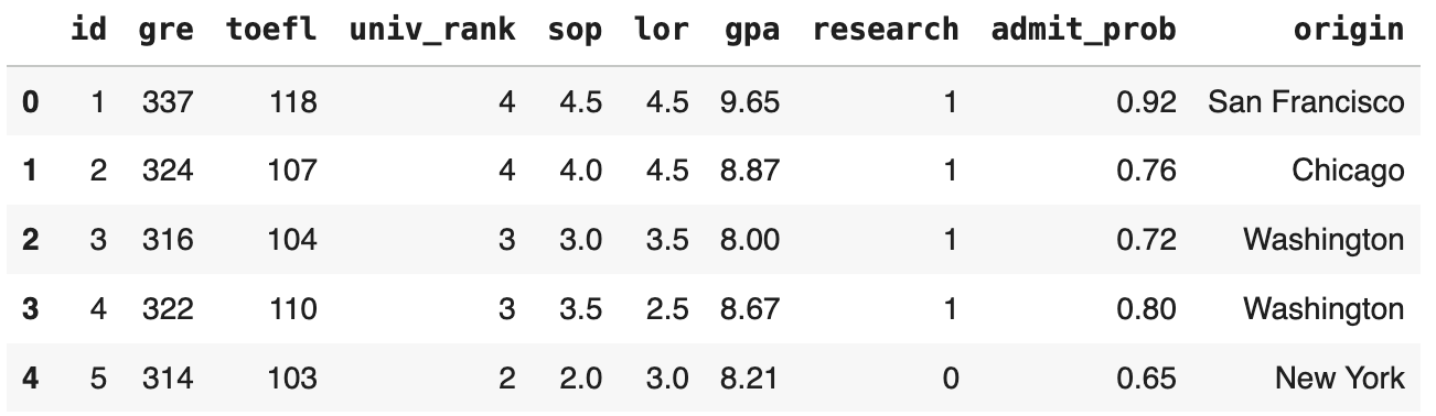

admission head (Image by Author)

Telco Customer Churn Data

This dataset will be used to represent classification modeling case.

# load dataset
import pandas as pd
churn = pd.read_csv("/path/to/WA_Fn-UseC_-Telco-Customer-Churn.csv")

# TotalCharges has object dtype; safely convert it to float
churn['TotalCharges'] = pd.to_numeric(churn['TotalCharges'], errors='coerce')

# label encode Churn column to binary
churn["Churn"] = churn["Churn"].apply(lambda x: 1 if x == "Yes" else 0)

# Churn head
churn.head()

churn head truncated (image by Author)

Regression model: choosing numeric features

To start this tutorial, we will consider our regression dataset (admission dataframe). This dataframe is rather simple, with only 10 columns and 400 rows.

admission dataframe info (Image by Author)

We will look at two methods for numerical feature selection in regression models: multicollinearity checks and F-regression tests.

Multicollinearity is the condition in which two or more features are strongly correlated. This is bad for modeling because it increases model variance and potential for overfitting, among other things (Yoo W, et al. 2014). Multicollinearity is model-agnostic. That is, regardless of the models we are dealing with, it is best to get rid of them.

The steps to perform feature selection via multicollinearity check are as follows:

1. Use only training data (to avoid data leak)
2. Find all sets of highly correlated features
3. For each of such set, retain only one feature that has the strongest correlation with the target variable

# get numeric column names
num_cols = admission.select_dtypes(include="number").columns.tolist()

# split train test data
from sklearn.model_selection import train_test_split

X = admission.drop("admit_prob", axis=1)
y = admission[["admit_prob"]]

X_train, X_test, y_train, y_test = train_test_split(X, y, test_size=0.2, random_state=42)

# multicollinearity check on training data
import matplotlib.pyplot as plt
import seaborn as sns

train_data = pd.concat([X_train, y_train], axis=1)

# correlation heatmap
plt.figure(figsize=(10, 8))
sns.heatmap(train_data[num_cols].corr(), annot=True)
plt.show()

admission’s feature correlation heatmap (Image by Author)

From the heatmap, we know that gre-toefl-gpa form a set of highly-correlated features (gre-toefl: 0.83; gre-gpa: 0.83, toefl-gpa: 0.82). We decide to retain gpabecause it has the strongest correlation with our target variabel (admit_prob) (gpa-admit_prob: 0.87; gre-admit_prob: 0.8; toefl-admit_prob: 0.78). In other words, we need to remove gre and toefl from both train and test data.

# drop gre and toefl columns (already covered by gpa)
X_train.drop(columns=["gre", "toefl"], inplace=True)
X_test.drop(columns=["gre", "toefl"], inplace=True)

For the second method, we will use the F-regression test. The purpose of this statistical test is to determine whether or not this numerical feature has a significant effect on the target variable.

For each numeric feature Xᵢ, it computes:

• The correlation between Xᵢ and target y
• Converts that correlation into an F-statistic (and p-value)

The F-statistic reflects how much that feature explains the variance of the target. I.e. if the F-statistic is large (associated with small p-value), then Xᵢ is informative and significant. And vice versa for small F-statistic (large p-value).

In our implementation, we’ll use SelectKBest function from the sklearn library to perform the F-regression test.

# updated numeric_cols
num_cols = X_train.select_dtypes(include=['int64', 'float64']).columns.to_list()

# feature selection using f_regression
from sklearn.feature_selection import SelectKBest, f_regression

selector = SelectKBest(f_regression, k=1)
selector.fit(X_train[num_cols], y_train.values.ravel())
pval_df = pd.DataFrame({
    'feature': num_cols,
    'p_value': selector.pvalues_
})

pval_df

p-values of F-regression test (Image by Author)

We can see that all numerical features are significant (p-value << 0.05), except for id column (p-value = 0.17 > 0.05), which is rather expected (Primary Key columns are generally non-informative for predicting the target variable). Therefore, we drop it.

# id feature is not significant, drop it
X_train.drop(column=["id"], inplace=True)
X_test.drop(column=["id"], inplace=True)

That is it. We have completed the feature selection of numeric columns for a regression model.

Regression model: choosing categorical features

To select categorical features for a regression model, we will use one-way ANOVA.

ANOVA is a statistical test that determines whether the means (averages) of multiple groups are statistically different. In our context, we use ANOVA to see if different categorical feature values result in statistically different means for the target variable (numeric).

SelectKBest does not natively support ANOVA for this scenario, so we need to write our own ANOVA function using the scipy library. The function is to be called within SelectKBest.

In the implementation below, note that we need to convert the categorical columns as numeric format first (we perform it via sklearn’s LabelEncoder).

# get categorical column names 
cat_cols = admission.select_dtypes(include="object").columns.tolist()

# concat X_train[categorical_cols] and y_train
cat_target = pd.concat([X_train[cat_cols], y_train], axis=1)
## cat_target = ["origin"]

# label encode origin column
from sklearn.preprocessing import LabelEncoder

le = LabelEncoder()
cat_target['origin'] = le.fit_transform(cat_target['origin'])

# define custom anova function
from scipy import stats

def categorical_anova_score(X, y):
    p_values = []
    for feature in X.T:
        # Group target values by categorical levels
        groups = [y[feature == val] for val in np.unique(feature)]
        # Perform one-way ANOVA
        _, p_val = stats.f_oneway(*groups)
        p_values.append(p_val)
    return np.array(p_values)

# Use with SelectKBest
from sklearn.feature_selection import SelectKBest

selector = SelectKBest(score_func=categorical_anova_score, k=1)
selector.fit(cat_target[cat_cols], y_train.values.ravel())
pval_df = pd.DataFrame({
    'feature': cat_cols,
    'p_value': selector.scores_
})

pval_df

origin’s ANOVA p-value (Image by Author)

We know that the origin feature has a very large p-value (>> 0.05), indicating that it has no effect on the target variable. So we drop it.

# origin is not significant, drop it
X_train.drop(columns=["origin"], inplace=True)
X_test.drop(columns=["origin"], inplace=True)

To summarize what we have done in our regression dataset (admission), we dropped the gre and toefl columns due to multicollinearity, and then dropped the id column because it had no significant influence on the target variable (admit_prob). On categorical feature side, we dropped origin column for the same reason as id (no significant effect on target variable).

Classification model: Choosing numeric features

Now we shift gear towards classification model (churn dataframe). This dataframe is more complex than admission. It has 21 columns (4 numeric, 17 categorical) with over 7000 rows.

churn dataframe info (Image by Author)

The first method we use to select numeric features is to check for multicollinearity. This is because, as previously stated, it is always best practice to eliminate multicollinearity in all modeling scenarios.

# get numeric column names
num_cols = churn.select_dtypes(include="number").columns.tolist()

# split train test data
from sklearn.model_selection import train_test_split

X = churn.drop("Churn", axis=1)
y = churn[["Churn"]]

X_train, X_test, y_train, y_test = train_test_split(X, y, test_size=0.2, random_state=42)

# multicollinearity check on training data
import matplotlib.pyplot as plt
import seaborn as sns

train_data = pd.concat([X_train, y_train], axis=1)

# correlation heatmap
plt.figure(figsize=(10, 8))
sns.heatmap(train_data[num_cols].corr(), annot=True)
plt.show()

churn dataset’s correlation (Image by Author)

From the heatmap, we know that tenure is highly correlated with TotalCharges (0.83). Between these two, we’ll retain tenure because it has larger absolute correlation (stronger) to our target variabel (Churn) (0.34 vs 0.19). In other words, we can remove TotalCharges.

# drop TotalCharges
X_train.drop(columns=["TotalCharges"], inplace=True)
X_test.drop(columns=["TotalCharges"], inplace=True)

For the next method, please observe that we want to assess effect of numerical features on a categorical target (classification). As a result, we can formulate the feature selection problem as follows: which numeric features have significantly different means for different target class values?

Sounds familiar? Yes, we can utilize one-way ANOVA for this.

Interestingly, SeleckKBest supports this ANOVA scenario (numeric features in classification model) natively via f_classif.

# updated numeric columns
num_cols = X_train.select_dtypes(include="number").columns.tolist()

# concat X_train[numeric_cols] and y_train
num_target = pd.concat([X_train[num_cols], y_train], axis=1)

# feature selection using f_classif (ANOVA)
from sklearn.feature_selection import SelectKBest, f_classif

selector = SelectKBest(f_classif, k=1)
selector.fit(X_train[num_cols], y_train.values.ravel())
pval_df = pd.DataFrame({
    'feature': num_cols,
    'p_value': selector.pvalues_
})

pval_df

churn’s numeric features ANOVA (Image by Author)

The results show that all remaining numerical features have a significant effect (p-value << 0.05) on the target variable (Churn), indicating that no additional numerical feature drops are required.

Classification model: Choosing categorical features

For the final scenario, we will use the Chi square test. This test determines the significance of a categorical feature is in influencing the categorical target variable by examining how the categorical feature values are distributed across different target class values. If the distributions differ significantly, we can keep the feature in our model (or vice versa).

SelectKBest does not directly support the Chi square test, so we must write a custom function to do it for us.

As with previous categorical features, we must first perform label encoding to convert the categorical columns to numerical values.

# get categorical column names
cat_cols = churn.select_dtypes(include="object").columns.tolist()

# concat X_train[categorical_cols] and y_train
cat_target = pd.concat([X_train[cat_cols], y_train], axis=1)

# label encode each categorical column
from sklearn.preprocessing import LabelEncoder

for col in cat_cols:
    le = LabelEncoder()
    cat_target[col] = le.fit_transform(cat_target[col])

# chi square test
from scipy.stats import chi2_contingency
import numpy as np

def chi2_score(X, y):
    n_features = X.shape[1]
    scores = np.zeros(n_features)
    # Calculate chi-square statistic for each feature
    for i in range(n_features):
        # Create contingency table
        contingency = pd.crosstab(X[:, i], y)
        # Perform chi-square test
        chi2, p_value, dof, expected = chi2_contingency(contingency)
        # Store the chi-square statistic as score
        scores[i] = p_value
    return scores

# Apply feature selection
selector = SelectKBest(score_func=chi2_score, k=1)
selector.fit(cat_target[cat_cols], y_train.values.ravel())
pval_df = pd.DataFrame({
    'feature': cat_cols,
    'p_value': selector.scores_
})

pval_df

churn data’s categorical features Chi square test(Image by Author)

From the results, we know that customerID, gender, and PhoneServiceare not significant (p-value > 0.05). Therefore, we can drop them.

# customerID, gender, PhoneService are not significant --> drop them
X_train.drop(columns=["customerID", "gender", "PhoneService"], inplace=True)
X_test.drop(columns=["customerID", "gender", "PhoneService"], inplace=True)

There you have it! We performed feature selection on the classification model case. We removed tenure to avoid multicollinearity (with TotalCharges). We also removed customerID, gender, and PhoneService due to their insignificant effect on the target variable (Churn).

Closing

In this article, we’ve been through a statistical framework to do feature selection in any modeling scenarios: modeling objectives vs feature types. All of the methods covered can be summarized as follows.

1. Regression model — numeric features: multicollinearity check & F-regression test
2. Regression model — categorical features: One-way ANOVA
3. Classification model — numeric features: multicollinearity check & One-way ANOVA
4. Classification model — categorical features: Chi square test

Hopefully, this will assist modeling practitioners and professionals alike in retaining only the best features from the available options in their machine learning models.

Finally, thanks for reading, and let’s connect with me on LinkedIn! 👋

References

https://en.wikipedia.org/wiki/Feature_selection

Yoo, W., Mayberry, R., Bae, S., Singh, K., He, Q. P., & Lillard Jr, J. W. (2014). A Study of Effects of MultiCollinearity in the Multivariable Analysis. International Journal of Applied Science and Technology, 4(5), 9–19. (accessed via this link)