Beyond TD(0): Exploring TD(1) and TD(λ) in Reinforcement Learning

In our previous post, we explored **Temporal Difference (TD) Learning (Check out the blog), with a special focus on TD(0)** — the simplest and most immediate form of value updating in reinforcement learning. But TD(0) is just one point on a broader spectrum.

To gain more flexibility and balance between short-term and long-term credit assignment, we introduce TD(1) and TD(λ) (TD-lambda), powerful generalizations that enhance learning stability and performance.

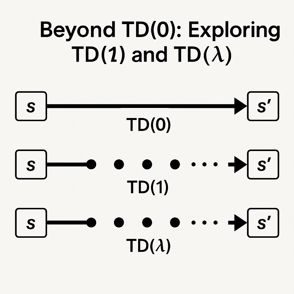
Figure 1 Beyond TD(0)

What is TD(1)?

While TD(0) updates value estimates using only the next state’s value (V(s′)), TD(1) goes to the other extreme—it updates based on the full return of an episode, similar to Monte Carlo methods.

In essence, TD(1) learns from the entire sequence of rewards, but still uses bootstrapping along the way.

Key Characteristics of TD(1):

• Waits until the end of the episode before updating values.
• Uses the actual return (sum of future discounted rewards).
• Equivalent to Monte Carlo in terms of outcome, but framed using TD’s bootstrapping style.

So why use TD(1) instead of Monte Carlo? Because TD(1) can still blend estimates and allow for online learning with some algorithmic tweaks, offering greater stability and flexibility.

The Power of TD(λ): A Unified View

Now let’s talk about TD(λ) (pronounced “TD-lambda”). This is where things get interesting.

TD(λ) generalizes both TD(0) and TD(1), allowing you to tune how much bootstrapping vs. full return you want. The λ (lambda) parameter ranges from 0 to 1:

• λ = 0 → behaves like TD(0)
• λ = 1 → behaves like TD(1) / Monte Carlo
• 0 < λ < 1 → a blend of short-term and long-term learning

Figure 2 The Power of TD(λ): A Unified View

This creates a spectrum of TD algorithms, where you can strike a balance between bias and variance, responsiveness and stability.

Why Use TD(λ)?

The real advantage of TD(λ) is that it provides:

• Faster convergence by leveraging longer reward traces.
• Stability through weighted updates.
• Control over credit assignment — how much of the final reward is “blamed” on earlier decisions.

This flexibility is crucial for complex environments where immediate feedback isn’t always informative, but waiting for the full return is inefficient.

How Does TD(λ) Work?

TD(λ) is often implemented using eligibility traces, which are temporary records that keep track of how recently each state (or action) was visited.

Each time the agent visits a state:

1. That state’s eligibility is increased.
2. Other states’ eligibilities decay.
3. The TD error (difference between predicted and actual outcome) is used to update all eligible states.

The more recently a state was visited, the more it is affected by the current TD error.

This mechanism lets the algorithm assign credit (or blame) proportionally across multiple time steps.

Real-World Analogy: Learning to Play Chess

Imagine teaching a beginner to play chess.

• TD(0): You give feedback after each move — whether it was good or bad — based on how the board looks immediately after.
• TD(1): You wait until the game ends, then tell them which early moves contributed to the win or loss.
• TD(λ): You give feedback that partially reflects both — the game result and how the position looked along the way, weighted by how recent each move was.

When to Use TD(0), TD(1), or TD(λ)

Use TD(0) when:

You need fast, online updates

Your environment changes rapidly

Immediate feedback is meaningful

Use TD(1) when:

You’re okay with waiting until the end of episodes

You want Monte Carlo-style learning with TD framing

Use TD(λ) when:

You want to balance long-term planning with short-term corrections

You want flexibility to tune performance

You’re working in complex, delayed-reward environments

Figure 3 When to Use TD(0), TD(1), or TD(λ)

Closing Thoughts

TD(λ) brings the best of both worlds. By blending TD(0) and TD(1), it allows agents to learn smarter — assigning credit in a way that’s more aligned with how real-world decisions often unfold. Whether you’re working on deep RL systems, games, or robotics, understanding and using TD(λ) can greatly improve your agent’s learning performance.

Stay tuned for the next post, where we’ll dive deeper into eligibility traces and how they power TD(λ) under the hood!