A Deep Dive into the Hessian Matrix

Before introducing the Hessian Matrix, it is important to first understand four foundational concepts: the eigendecomposition of symmetric matrices, the properties of positive definite matrices, the convexity and concavity of functions, and Newton’s method in optimization.

1. Eigendecomposition of symmetric matrices

Please refer to my article about the eigendecomposition of symmetric matrices.

TL;DR A symmetric matrix can be eigendecomposed to A=QΛQᵀ, where Λ is the diagonal matrix of eigenvalues and Q is the orthogonal matrix of eigenvectors.

2. Positive Definite Matrix

Definition: A real symmetric matrix A is positive definite if it satisfies the positive quadratic form all nonzero vector x, that is, xᵀAx > 0.

Key Properties of Positive Definite Matrix:

• Real and Symmetric The requirement for symmetry is because a non-symmetric matrix satisfying xᵀAx > 0 for all nonzero vectors x might not have all real eigenvalues. In contrast, a symmetric matrix that satisfies xᵀAx > 0 for all nonzero vectors x is guaranteed to have all real eigenvalues. This can be proven using complex numbers and conjugate operations.
• Full-rank and invertible
• All eigenvalues of the matrix are positive. Proof: If λᵢ is the eigenvalue corresponding to the eigenvector vᵢ​ of a matrix A, then it satisfies Avᵢ​ = λᵢ​vᵢ. Also, as the quadratic form is positive in the positive definite matrix, vᵢ​ᵀAvᵢ​ = λᵢvᵢ​ᵀvᵢ​ = λᵢ ||​vᵢ||² > 0. Hence, λᵢ > 0, that is, each eigenvalue of the matrix is positive.
• The determinant of the matrix is positive, det(A) > 0. Proof: det(A) = λ₁λ₂…λₙ > 0 I will leave the complete proof process to you :)
• Condition number of the matrix = λₘₐₓ / λₘᵢₙ

Similar Concepts

• Positive (Semi)Definite Matrix: All eigenvalues are positive (or zero).
• Negative (Semi)Definite Matrix: All eigenvalues are negative (or zero).
• Indefinite Matrix: Has both positive and negative eigenvalues.

3. Convexity, Concavity, and Curvature

You can refer to my article about convexity, concavity, and curvature of the function’s graph.

TL;DR

1. In 2D, second-derivative f ′′(x), along with curvature, can provide information about the concavity of a function’s graph: a) When f ′′(x) > 0, the function is concave up (U-shape) b) When f ′′(x) < 0, the function is concave down (∩-shape)
2. In 3D, we use the Hessian matrix, formed by all the second partial derivatives (∂²f / ∂x², ∂²f / ∂y², ∂²f / ∂x∂y), to analyze the concavity of the function’s graph in 3D and higher dimensions.

4. Newton’s Method in Optimisation

Newton’s Method for Root Finding

The Newton method is an iterative technique for finding roots of a function f (x) = 0.

Using the first-order Taylor series expansion, we can approximate the f (x) near xₙ: f (x) ≈ f (xₙ) + f ′(xₙ)(x - xₙ). Setting f (x) = 0 for root finding, we get: 0 ≈ f (xₙ) + f ′(xₙ)(x - xₙ). Hence, the next iteration xₙ₊₁ = xₙ - f (xₙ)/f ′(xₙ).

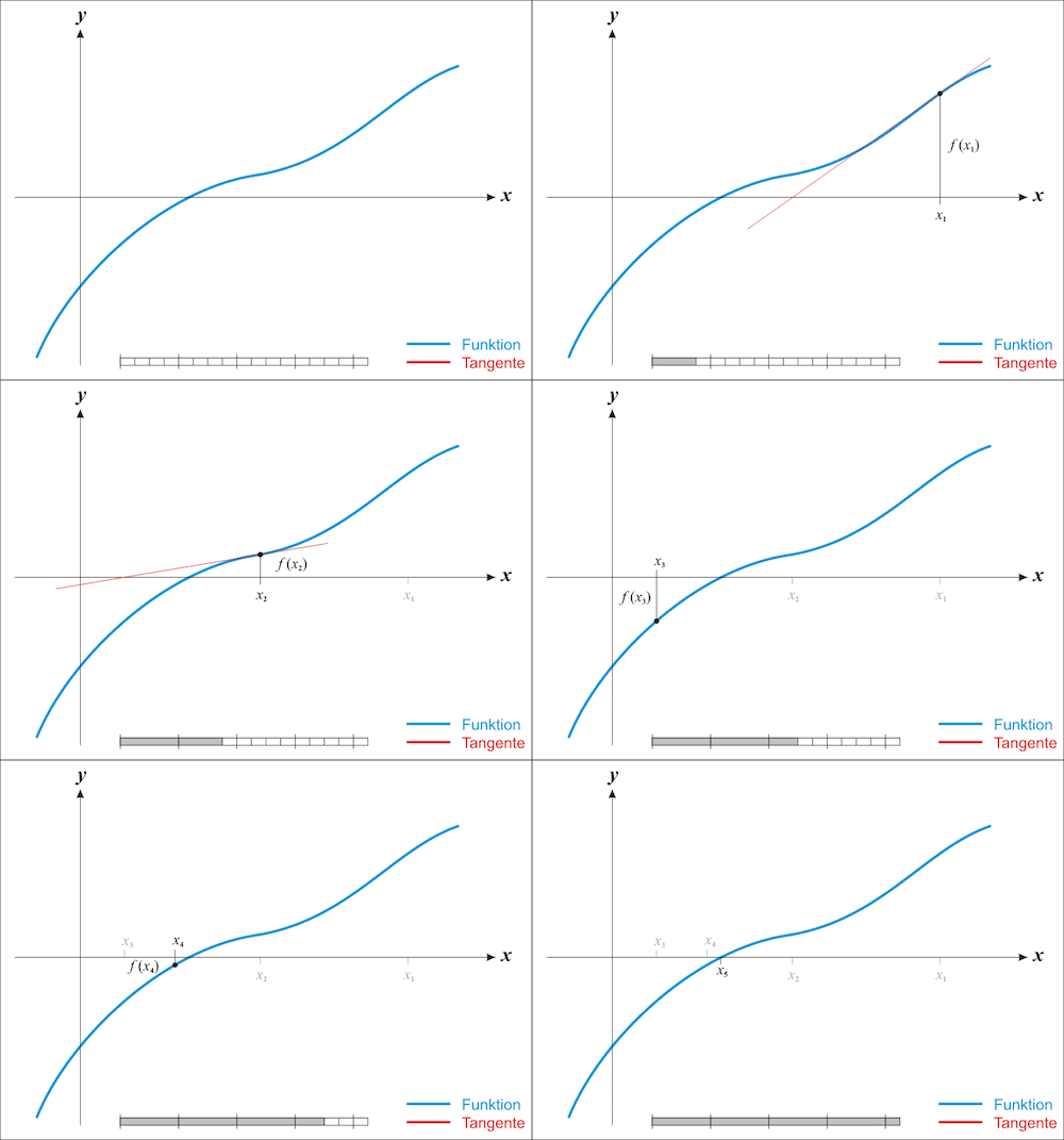
Fig. 1. Newton Method for Iterative Root Finding (image from Wikipedia)

Newton’s Method in Optimisation

If function f (x) is twice differentiable, we can use Newton’s method on its derivative 𝑓′(x) to find solutions to 𝑓′(x) = 0, also known as the critical points of f (x). These solutions may be minima, maxima, or saddle points.

Using the second-order Taylor series expansion, we can approximate the f (x) near xₙ: f (x) ≈ f (xₙ) + f ′(xₙ)(x - xₙ) + 1/2 f ′′(xₙ)(x - xₙ)². Setting f ′(x) = 0 for the critical point, we get: 0 ≈ f ′(xₙ) + f ′′(xₙ)(x - xₙ). Hence, the update rule is given by: xₙ₊₁ = xₙ - f ′(xₙ)/f ′′(xₙ).

Newton’s Method v.s. Gradient Descent in Optimisation

• Gradient Descent: the update rule is xₙ₊₁ = xₙ - εf ′(xₙ), where ε is the learning rate, εf ′(xₙ) is the step size.
• Newton’s method: the update rule is xₙ₊₁ = xₙ - f ′(xₙ)/f ′′(xₙ), where f ′(xₙ)/f ′′(xₙ) is the step size, incorporating the curvature information (i.e. the second derivative) in contrast to Gradient Descent.

The key advantage of Newton’s method is its ability to adjust step size based on the local shape of the function, without manual tuning of a learning rate parameter ε. This adaptive step size allows: a. When the function is relatively flat, low curvature where f ′′(xₙ) is small, the step size becomes larger. b. When the function changes rapidly, high curvature where f ′′(xₙ) is large, the step size becomes smaller.

Fig. 2. A comparison of gradient descent (green) and Newton’s method (red) for minimizing a function f(x). Newton’s method uses curvature information to take a more direct route. (image from Wikipedia)

Now let’s talk about the Hessian Matrix. It should be much easier with the establishment of these three foundational concepts.

Hessian Matrix

Definition: Hessian matrix H is a square matrix of second-order partial derivatives of a scalar-valued function f(x), x ∈ ℝⁿ.

Furthermore, if the second partial derivatives of f(x) are all continuous, the second derivatives are symmetric (∂²f / ∂xᵢ ​∂xⱼ = ∂²f / ∂xⱼ∂xᵢ ​), hence the Hessian matrix is symmetric.

According to the first foundational concept, Eigendecomposition of Symmetric Matrices, Hessian matrix H can be eigendecomposed to H=QΛQᵀ, where Λ = diag(λ₁, λ₂, …, λₙ).

By checking the sign of all eigenvalues and using the second foundational concept, Positive Definite Matrix, we can get the following:

• If all eigenvalues are positive, then H is positive definite.
• If all eigenvalues are negative, then H is negative definite.
• If eigenvalues have both positive and negative values, then H is indefinite.

Hessian Matrix Application 1: Second-derivative Test

When given a critical point 𝑥, where the gradient at this point is zero (f ′(x) = 0 or ∇f (𝑥)*= *0), we can use properties of Hessian Matrix H to test whether 𝑥 is a local maximum, local minimum, or a saddle point, as follows:

• If Hessian matrix H(𝑥) is positive-definite (all eigenvalues are positive), then f (𝑥) attains a strict local minimum at 𝑥.
• If the Hessian matrix H(𝑥) is negative-definite (all eigenvalues are negative), then f (𝑥) attains a strict local maximum at 𝑥.
• If the Hessian matrix H(𝑥) is indefinite (eigenvalues have both positive and negative values), then 𝑥 is a saddle point of f (𝑥).
• If the Hessian matrix H(𝑥) is degenerate (one of the eigenvalues is zero, det(H(𝑥)) = 0), then the second-derivative test is inconclusive, meaning we can’t decide if 𝑥 is a local maximum, local minimum, or a saddle point.

Fig. 3. Different Types of Critical Points: a) Local Minimum, b) Local Maximum, c) Saddle Point, and their Corresponding Eigenvalues for the Hessian Matrix of the Function. (image by author)

The eigenvalues of a function’s Hessian matrix correspond to the second-order derivatives along the principal directions (eigenvectors), indicating the concavity of the function in those directions.

In higher-dimensional spaces (n > 3), although visualization becomes challenging, the second derivative test remains valid.

Hessian Matrix Application 2: Optimization

In the fourth foundational concept, Newton’s Method in Optimisation, is about single variable functions. Now let’s discuss the case of multiple dimensions.

Newton’s Method in Multi-Dimensional Optimisation

Using the second-order Taylor series expansion, we can approximate the f (x) near xₙ: f (x) ≈ f (xₙ) + ∇f (xₙ)(x — xₙ) + 1/2 (x — xₙ)ᵀ H(xₙ) (x — xₙ). Setting ∇f (x) = 0 for the critical point, we get: 0 ≈ ∇f (xₙ)+ H(xₙ)(x — xₙ). Hence, the update rule is given by: xₙ₊₁ = xₙ — H(xₙ)⁻¹∇f (xₙ).

Newton’s Method v.s. Gradient Descent in Multi-Dimensional Optimisation

• Gradient Descent: the update rule is xₙ₊₁ = xₙ — ε∇f (xₙ), where ε is the learning rate and ε∇f (xₙ) is the step size.
• Newton’s method: the update rule is xₙ₊₁ = xₙ — H(xₙ)⁻¹∇f (xₙ), where H(xₙ)⁻¹∇f (xₙ) is the step size, incorporating the curvature information (Hessian matrix formed by the second derivative) in contrast to Gradient Descent.

Advantages of Newton’s Method

The advantage of Newton’s method is its ability to adjust step size based on the local curvature, while Gradient Descent fails to exploit the curvature information, especially when the Hessian matrix has a high condition number, leading to oscillatory behavior and slower convergence.

(Note: In multiple dimensions, a high condition number of the Hessian matrix indicates that the function has significantly different second derivatives in different principle directions. Some directions have high curvature, while others have low curvature.)

Fig. 4. Gradient descent fails to exploit the curvature information in the Hessian matrix with a high condition number. (image from <Deep Learning> by Ian Goodfellow)

Disadvantages of Newton’s Method

1. In deep learning neural networks, the objective function is typically non-convex and high-dimensional (e.g., millions of parameters). In such high-dimensional spaces, critical points are more likely to be saddle points rather than local minima. This is due to the probability of all eigenvalues of the Hessian matrix being positive (indicating a local minimum) becoming increasingly small as dimensionality grows. While Newton’s method is designed to converge to the critical point, since the critical points are most likely saddle points as mentioned, Newton’s method is more likely to be attracted to saddle points rather than true local minima.
2. Newton’s method is computationally expensive for training large neural networks. With n parameters (which could be millions or even billions in modern deep learning models), the space complexity of storing the Hessian matrix is O(n²), and the time complexity of inverting the Hessian matrix is O(n³).

Takeaway:

1. Newton’s method is an excellent tool for minimizing convex functions (the Hessian matrix is positive semidefinite), especially when the Hessian matrix is poorly conditioned (with a high condition number).
2. In deep learning models consisting of nonconvex optimization problems, Newton’s method is likely to be attracted to saddle points rather than true local minima and is computationally expensive. For these reasons, pure Newton’s method is rarely used in deep learning.
3. First-order methods like Stochastic Gradient Descent (SGD) and its variants (e.g., Adam, RMSprop) are the go-to algorithms for the training process. They are less likely to get stuck at saddle points and are computationally more efficient.