Multi-GPU Training Explained: Data Parallelism, Input Sharding, and Performance Trade-offs (Part 1)

A practical guide to scaling deep learning models with multi-GPU data parallelism, covering core concepts, memory bottlenecks, and real-world performance considerations

Photo by Nicki Eliza Schinow on Unsplash

Model training has become extremely resource-intensive as model size and dataset volumes grow exponentially. GPU memory and compute capacity — determined by core count and clock speed — aren’t scaling at the same pace as data and model requirements. This gap forces machine learning practitioners to adopt multi-GPU configurations for training modern neural networks.

In this guide, we’ll explore how to effectively train models in multi-GPU environments. You’ll learn different parallelization strategies and practical implementations for distributed training setups. This content is designed for readers with foundational machine learning knowledge.

This two-part series is structured as follows:

• Part 1 (this article) focuses on the fundamentals: introduction to multi-GPU training concepts, input sharding techniques, and hands-on coding examples.
• Part 2 (coming 13 Feb 20206) covers model sharding approaches, with emphasis on training large language models (LLMs) and vision-language models (VLMs).

Why Multi-GPU Training Is Essential for Modern Deep Learning?

Over a decade ago, GPUs revolutionized model training by leveraging CUDA cores for parallel computing. As computational demands scaled, GPU memory emerged as the primary bottleneck. While NVIDIA’s latest GPU models attempted to address these limitations, they couldn’t keep pace with exponentially growing requirements. Here are the core challenges that make single-GPU training impractical today:

1. Larger Models Exceed GPU Memory Limits: Modern models have outgrown even the most powerful GPUs. DeepSeek V2, for instance, requires approximately 236 GB of storage, while the largest commercially available GPU VRAM tops out at 192 GB (NVIDIA’s Blackwell series).
2. Training Overheads Multiply Memory Requirements: Training large models demands far more than just loading model weights. Memory-intensive overheads — including gradients, optimizer states, and activations — must be stored during training. For pretraining scenarios, these accumulated overheads often consume more memory than the model weights themselves.
3. Dataset Sizes Have Exploded: Training data continues to grow massively. Even a compact detection model like YOLOv11s (under 100 MB) requires the ImageNet dataset, which exceeds 150 GB. Larger, more sophisticated models demand proportionally larger datasets.
4. Complex Models Demand Larger Batch Sizes: Different architectures require specific batch sizes for optimal convergence. Vision-language models and large language models (LLMs) typically need very large batch sizes to converge effectively, further straining already overloaded GPU memory.
5. Single-GPU Training Is Prohibitively Slow: While workarounds exist to train models on single GPUs despite the above limitations, training time becomes impractically long. Multi-GPU configurations are often the only viable path to reasonable training speeds.

The Core Issue: Memory, Not Compute

These challenges reveal that GPU memory capacity — not computational power — is the fundamental bottleneck for modern model training. The data and model sizes we need to handle vastly exceed what current GPU memory can store. Since increasing physical GPU memory presents significant hardware challenges, recent innovations have focused on algorithmic solutions: efficiently loading and unloading data across multiple GPUs. Let’s explore how multi-GPU training addresses these limitations at the algorithmic level.

Data Sharding: Distributing Training Data Across GPUs

Data sharding encompasses methods for dividing datasets across multiple GPUs. This widely-adopted approach for multi-GPU training benefits from robust library support and active community adoption. Since these methods don’t require specialized hardware — just fast SSDs and GPUs — practitioners can achieve significant performance gains immediately. Let’s explore how data sharding works in practice.

Data Parallel Training: The Foundation of Multi-GPU Scaling

Data parallelism is the most common and intuitive strategy for scaling deep learning training. The fundamental concept is straightforward: perform backpropagation by distributing data across multiple GPUs. This approach works effectively when your model and its training intermediate states (gradients, optimizers, activations, etc.) fit comfortably within a single GPU’s memory. Here’s how the process works step-by-step.

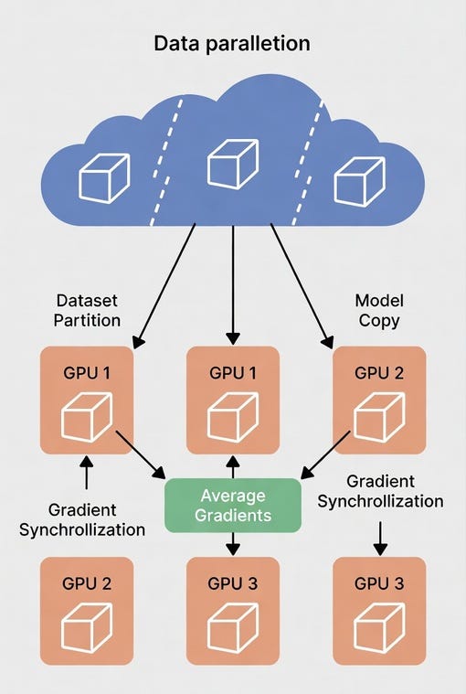
Algorithm Breakdown

1. Load Model — Each GPU receives an identical copy of the model
2. Data Sharding — The dataset is partitioned into N non-overlapping subsets, where N equals the number of GPUs. This ensures each GPU processes a unique data portion with zero duplication. PyTorch’s Distributed Sampler handles this implementation.
3. Forward Pass — Each GPU’s model performs a standard forward pass on its assigned data subset
4. Backward Pass — Each GPU independently calculates its own gradients
5. Synchronization — GPUs communicate to compute average gradients across all devices. This uses the “all reduce” algorithm implemented via the NCCL library.
6. Parameter Update — Model parameters update using the averaged gradients. Since all models started with identical weights and were updated with identical gradients, they maintain weight synchronization after the update.

Scaling Beyond Single Nodes

The approach described above applies to single-node, multi-GPU training. For larger-scale training, this algorithm extends to multi-node clusters. The core logic remains unchanged, with added communication overhead between nodes. This distributed training method is called Distributed Data Parallel (DDP). The original Data Parallel implementation used a single orchestrating GPU, creating significant overhead on one device. The current approach eliminates this bottleneck.

Advantages of Data Parallel Training

1. Near-linear scaling: Adding a second GPU typically delivers 1.8x to 1.9x speedup
2. No Python GIL issues: Each GPU runs as a separate process, avoiding Global Interpreter Lock constraints
3. Framework compatibility: Works seamlessly with wrappers like PyTorch Lightning and Hugging Face Accelerate
4. Minimal code changes: Transitioning from single-GPU to multi-GPU requires minimal modifications
5. Horizontal scalability: Easily scales from 2 GPUs to hundreds of devices

Limitations to Consider

1. Model size constraint: Cannot train models larger than the single GPU memory capacity
2. Synchronization overhead: Gradient synchronization introduces significant communication costs
3. Memory redundancy: Substantial GPU memory is wasted replicating models across devices

Beyond Neural Networks

Data parallelism extends beyond deep learning. Classical machine learning models — including clustering algorithms, linear regression, and others — leverage data parallelism extensively for distributed training.

Now that we’ve covered the theoretical foundations, let’s examine the programming implementation for data parallel training.

import torch
import torch.nn as nn
import torch.distributed as dist
from torch.utils.data import DataLoader, DistributedSampler
from torch.nn.parallel import DistributedDataParallel as DDP
import torchvision.datasets as datasets
import torchvision.transforms as transforms
import os

# ─── 1. Initialize the process group ────────────────────────────
def setup(rank, world_size):
    os.environ["MASTER_ADDR"] = "localhost"
    os.environ["MASTER_PORT"] = "12355"
    dist.init_process_group(backend="nccl", rank=rank, world_size=world_size)

# ─── 2. Define a simple model ────────────────────────────────────
class SimpleModel(nn.Module):
    def __init__(self):
        super().__init__()
        self.fc = nn.Sequential(
            nn.Linear(784, 256),
            nn.ReLU(),
            nn.Linear(256, 10)
        )

    def forward(self, x):
        return self.fc(x.view(x.size(0), -1))

# ─── 3. Create DataLoader with DistributedSampler ───────────────
def get_dataloader(rank, world_size, batch_size=64):
    dataset = datasets.MNIST("./data", train=True, download=True,
                             transform=transforms.ToTensor())
    sampler = DistributedSampler(dataset, num_replicas=world_size, rank=rank)
    return DataLoader(dataset, batch_size=batch_size, sampler=sampler)

# ─── 4. Training loop ────────────────────────────────────────────
def train(rank, world_size, epochs=5):
    setup(rank, world_size)

    device = torch.device(f"cuda:{rank}")
    model = SimpleModel().to(device)
    model = DDP(model, device_ids=[rank])          # Wrap with DDP

    dataloader = get_dataloader(rank, world_size)
    optimizer = torch.optim.Adam(model.parameters(), lr=1e-3)
    criterion = nn.CrossEntropyLoss()

    for epoch in range(epochs):
        dataloader.sampler.set_epoch(epoch)        # Shuffle differently each epoch
        for batch_idx, (data, target) in enumerate(dataloader):
            data, target = data.to(device), target.to(device)

            optimizer.zero_grad()
            output = model(data)
            loss = criterion(output, target)
            loss.backward()                        # Gradients auto-synced by DDP
            optimizer.step()

        if rank == 0:                              # Print only from rank 0
            print(f"[Epoch {epoch+1}] Loss: {loss.item():.4f}")

    dist.destroy_process_group()

# ─── 5. Launch ────────────────────────────────────────────────────
if __name__ == "__main__":
    world_size = torch.cuda.device_count()        # Number of GPUs available
    torch.multiprocessing.spawn(train, args=(world_size,), nprocs=world_size, join=True)

Similarly, we can also leverage the Dask library for multi-GPU training for linear regression (classical ML) using the example code given below.

import cupy as cp
import dask.array as da
from dask_ml.linear_model import LinearRegression
from dask_cuda import LocalCUDACluster
from dask.distributed import Client

def main():
    # Start Dask GPU cluster
    cluster = LocalCUDACluster()
    client = Client(cluster)

    # Create synthetic data on GPUs
    X = da.random.random(
        (1_000_000, 10),
        chunks=(100_000, 10),
        asarray=cp.asarray
    )
    y = X.sum(axis=1) + 0.1 * da.random.random(
        1_000_000,
        chunks=100_000,
        asarray=cp.asarray
    )

    # Distributed multi-GPU model
    model = LinearRegression()

    # Train (distributed across GPUs)
    model.fit(X, y)

    print("Training complete")
    print("Coefficients:", model.coef_)

    client.close()

if __name__ == "__main__":
    main()

Context Parallelism: Scaling LLMs to Handle Massive Sequence Lengths

The attention block represents the primary computational bottleneck in large language models (LLMs). This bottleneck stems from attention’s quadratic (exponential) relationship with sequence length. As context windows expand, memory requirements for processing larger contexts grow exponentially. Context parallelism solves this by sharding input across multiple GPUs for independent parallel processing.

The Problem: Attention Memory Footprint

The core challenge is fitting gigantic attention matrices into GPU memory. Context parallelism addresses this by breaking input into manageable sub-sections, running attention computations on each subsection independently, then aggregating results. By reducing sequence size through partitioning, we dramatically decrease computational costs.

Algorithm Breakdown

Step 1: Sequence Partitioning

The input sequence is divided into multiple chunks distributed across GPUs. All attention module components — including K (Key), Q (Query), and V (Value) matrices — are shared alongside the input sequence. Sharding can occur across any number of dimensions.

Example partitioning:

• Total tokens: [0, 1, 2, …, 1023]
• GPU 0: processes tokens [0–255]
• GPU 1: processes tokens [256–511]
• GPU 2: processes tokens [512–767]
• GPU 3: processes tokens [768–1023]

Step 2: Local Attention Calculation

Each GPU calculates attention independently using its assigned data partition.

Step 3: Combining Partial Outputs Using Ring Attention

This critical step aggregates results across all GPUs through a ring-based communication pattern:

1. Each GPU calculates attention and passes results to the next GPU in the ring
2. Simultaneously, each GPU receives computed results from the previous GPU
3. This ring structure enables theoretically infinite context length processing (refer to Ring Attention research for a deeper understanding)

Step 4: Backward Pass Through the Ring

Once Steps 2 and 3 are complete, the forward pass, and the backward pass begins in reverse order. Gradients accumulate following the same ring pattern. Note that backward passes are often computationally expensive.

Advantages of Context Parallelism

1. Extended context handling: Processes context lengths far exceeding single GPU memory capacity
2. Scalable architecture: Grows efficiently with additional GPUs
3. No pipeline bubbles: Maintains high GPU utilization throughout training

Limitations to Consider

1. Intra-GPU bottleneck dependency: Performance constrained by inter-GPU communication speeds
2. Ring attention overhead: Additional computational cost from the ring communication pattern
3. Load balancing complexity: Requires input sequence-based balancing strategies, which can be challenging

Implementation in Practice

Below is basic introductory code for context parallelism. In production environments, context parallelism typically integrates into larger pipelines combining multiple parallelism strategies and optimizations through established frameworks.

import torch
from accelerate import Accelerator
from accelerate.utils import DistributedDataParallelKwargs
from torch.utils.data import DataLoader, TensorDataset

def train_long_context():
    # 1. Initialize Accelerator with CP enabled
    # 'cp_size' defines how many GPUs work together on a single sequence
    accelerator = Accelerator(
        kwargs_handlers=[DistributedDataParallelKwargs(gradient_as_bucket_view=True)]
    )

    # 2. Setup a dummy model (e.g., a Transformer)
    model = torch.nn.Transformer(d_model=512, nhead=8).to(accelerator.device)
    optimizer = torch.optim.AdamW(model.parameters(), lr=1e-5)

    # 3. Create long-sequence data (e.g., 32k tokens)
    # Batch size of 1, but sequence length is massive
    input_data = torch.randn(1, 32768, 512) 
    dataset = TensorDataset(input_data)
    loader = DataLoader(dataset, batch_size=1)

    model, optimizer, loader = accelerator.prepare(model, optimizer, loader)

    # 4. Use the Context Parallel manager
    # This automatically shards the buffers (input_data) along dimension 1 (sequence)
    for batch in loader:
        with accelerator.context_parallel(
            buffers=[batch[0]], 
            buffer_seq_dims=[1]
        ):
            # Each GPU now only processes (32768 / num_gpus) tokens
            output = model(batch[0], batch[0])
            loss = output.mean()

            accelerator.backward(loss)
            optimizer.step()
            optimizer.zero_grad()

    print(f"Rank {accelerator.process_index} finished iteration.")

if __name__ == "__main__":
    train_long_context()

Conclusion

We have explored the fundamentals of distributing input data across multiple GPUs to overcome the “memory wall” of modern hardware. By transitioning from single-device setups to distributed environments, we can scale our workloads to meet the demands of increasingly complex architectures.

Key Takeaways:

• Data Parallelism: The standard approach for traditional deep learning (non-Generative AI) models and classical AI models. It allows for near-linear scaling by replicating the model and sharding the dataset.
• Context Parallelism: An essential strategy for modern, large-scale Generative AI models. It enables the processing of massive sequence lengths by sharding the attention mechanism itself across the GPU cluster.

What’s Next? In our next post, we will dive into Model Sharding. We will examine how to partition a model’s parameters across multiple GPUs, a critical requirement for training today’s multi-billion parameter LLMs and VLMs.

Thank you for reading!

From the Author: Apurva Bhatt

If you found this article insightful and beneficial, please consider following me and leaving a clap for more in-depth content! Your support helps me continue producing content that aids our collective understanding.