Can Protein Function Be Learned From Network Structure Alone?

Exploring DeepWalk and Node2Vec on Protein Interaction Networks from Scratch

Before graph neural networks became popular, graph data representation learning was driven by the concept of random walks and embedding methods such as DeepWalk and Node2Vec which were inspired by word embedding models like Word2Vec (Skipgram).

These methods were developed to answer the question.

Can graph topology alone produce meaningful vector representations?

In this article I will explore the Protein–Protein Interaction (PPI) dataset to create the node embeddings directly from graph topology. The goal is to understand how graph topology can be converted into meaningful protein representations/embeddings

Protein-Protein Interaction Dataset

Protein-Protein interaction network happens when two or more proteins work together to perform a biological function naturally forming a graph structure. It originates from the Predicting multicellular function through multi-layer tissue networks paper and is structured specifically for multi-label node classification

Nodes -> Individual Protein

Edges -> Interaction/Connection between proteins

The complete PPI dataset

Total Number of graphs in PPI dataset -> 24

Average Number of nodes per graph -> ~2245

Average Number of edges per graph -> ~61318

Number of node features -> 50 containing positional gene sets, motif gene sets and immunological signatures as features

For our experiment we sample one random graph for further exploration with following properties

the sampled graph contains

• 1767 proteins
• 50 node features per protein
• 32318 protein interactions
• 121 multi label annotations for each protein because each protein can have multiple functions

Exploratory Data Analysis: Graph Topology

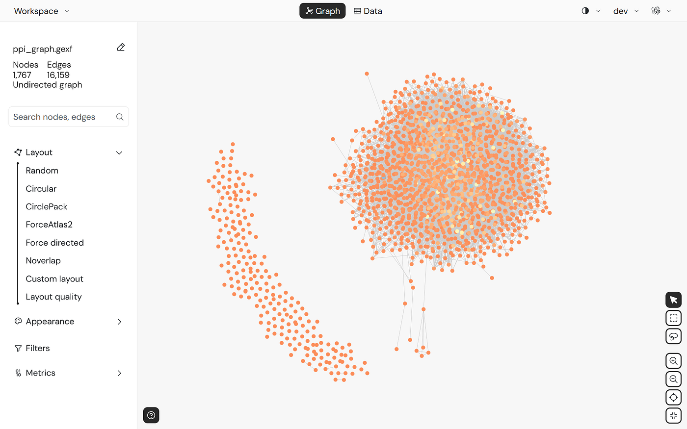
Visualizing one of the graphs using Gephi Software we see that the node connectivity (degree of connection) varies significantly ranging from 0 (isolated nodes) to highly connected nodes with 286 connections

For example the protein node 1536 with degree 3, the neighbours are 144, 905 and 885. The goal of graph embeddings is to capture this topological information.

degrees = dict(G.degree())

print(f"Minimum Degree connectivity {min(degrees.values())}")
print(f"Maximum Degree connectivity {max(degrees.values())}")

count_degrees = Counter(degrees)

print(f"Top3 nodes with highest connectivity")
topnodes =count_degrees.most_common(n=3)

for node, degree in topnodes:
    print(f"Node: {node}, Degree of connectivity: {degree}")
==================================================================
Minimum Degree connectivity 0
Maximum Degree connectivity 286
Top3 nodes with highest connectivity
Node: 1449, Degree of connectivity: 286
Node: 613, Degree of connectivity: 257
Node: 495, Degree of connectivity: 243

There are also some isolated proteins that do not connect with any other proteins

isolated_nodes = list(nx.isolates(G))

print("Number of isolated nodes:", len(isolated_nodes))
print(isolated_nodes[:10])
=========================================================================
Number of isolated nodes: 209
[282, 486, 892, 1030, 1060, 1204, 1250, 1405, 1554, 1555]

DeepWalk.

The goal of DeepWalk was to generate feature representations that are used by other models for different tasks such as classification. DeepWalk is heavily inspired by Word2Vec, but in our case the dataset is composed of nodes rather than words. DeepWalk is a simple baseline that can be implemented quickly to graph data. To make the graph dataset behave like a sentence in Word2Vec, we use uniform random walks for creating a meaningful sequence of nodes. Random walks are nothing but randomly sampling a neighbouring node at each step.

In random walk, we will start with say node 1536, from its neighbours select any one neighbour say 144 and so on till we reach the desired length. One interesting case in our dataset is the presence of isolated proteins.

In many graphs, connected or nearby nodes often share similar properties or roles so if nodes often appear together in a random walk sequence, it means they are similar. The idea behind DeepWalk is that we want the nodes close to each other to have similar embedding as compared to nodes that are rarely together.

Implementing DeepWalk

We first start by creating random walks of We start with a start node and at every step select a random neighbouring node until walk is complete.

def random_walk(start_node, G,walk_length=10):
    walk = [start_node]
    for _ in range(walk_length):
        neighbours = list(G.neighbors(start_node))
        next_node = int(np.random.choice(neighbours, 1)[0])
        walk.append(next_node)
        start_node = next_node
return [str(x) for x in walk]

let us look at random walk of size 10, where start node is 0

random_walk(start_node=0,G=G,walk_length=10)
['0', '766', '611', '1051', '1218', '613', '502', '1355', '884', '1095', '889']

now let us extend this unbiased random walks to all nodes with walk length of 20 and 50 times each for each node to create our dataset

walks = []
for node in G.nodes:
    walks.extend([random_walk(node,G,20) for _ in range(50) if node not in isolated_nodes])

Preprocessing Note: Before generating random walks isolated nodes were filtered from the graph to avoid walks containing only the source node. An isolated node has no neighbour so any random walk starting there would get trapped resulting in noise in the dataset

model  = Word2Vec(walks,vector_size=256,window=10,
                   sg =1, hs=1,seed=0,
                 workers=os.cpu_count()-1) # type: ignore

model.train(walks, total_examples=model.corpus_count,
            epochs=20,
            report_delay=True,
            compute_loss=True)

Analyzing DeepWalk Embeddings

let us now look at node with id “0” and its first 10 embeddings

model.wv[str(0)][:10]
array([ 0.25209188, -0.21169102, -0.22076103,  0.3142252 , -0.14155613,
 -0.11256588,  0.36132765,  0.27915508,  0.3109536 , -0.20226778],
 dtype=float32)

After training DeepWalk, every protein node is converted into a dense vector representation called an embedding and DeepWalk learns these embeddings directly from graph structure. These embeddings capture structural information.

But does this representation capture structure?

Let us look at the actual direct neighbors of node 0 compared to its top 5 most similar nodes in the embedding space

For node 0 its neighbours are 372, 1101, 766

print("True Neighbors:", list(G.neighbors(0)))
print("Top 5 Most Similar Embeddings:\n", model.wv.most_similar(positive=['0'], topn=5))
[372, 1101, 766]

True Neighbors: [372, 1101, 766]
Top 5 Most Similar Embeddings:
[('766', 0.5627827048301697),
 ('372', 0.49181830883026123),
 ('1101', 0.4064106047153473),
 ('1489', 0.3511863946914673),
 ('352', 0.3417294919490814)]

The model assigns highest cosine similarity to its 1st degree or immediate neighbours and if we see how the other 2, nodes 1489 and node 352 are connected using the shortest path.

print(nx.shortest_path(G,0,352))
print(nx.shortest_path(G,0,1489))

[0, 1101, 352]
[0, 766, 1489]

Although nodes 352 and 1489 are not direct neighbors of node 0 but at a degree connectivity of 2, they are only two hops away in the graph meaning that although the nearest neighbours have high similarity score, there are nodes which may not be directly connected but they often appear together in random walks.

We can also measure similarity between proteins using cosine similarity between embeddings. Proteins with similar embeddings often occupy similar positions in the graph.

Biased Random Walks and Node2Vec

Node2Vec extends the idea of DeepWalk by introducing biases in random walks. Instead of uniformly sampling the next neighboring node, Node2Vec controls the random walk behaviour using transition probabilities. This allows the random walks to either remains close to the local neighbourhood of a node or explore further regions within the graph structure.

Suppose the current node is b, and the previous node is a, the unnormalized transition probability from current node b to next c is

*Πbc = α(a,c) w(b,c) where α(a,c) is the search bias between nodes a and c and w(b,c) is the weight of edge from b,c. In DeepWalk α(a,c) =1**. In Node2vec the value of α(a,c) depends upon

Return Parameter (p): controls the probability of revisiting the previous node. Lower values of p increase the likelihood of returning back to the previous node

In-out Parameter (q): controls the probability or exploring the further. Lower values of q encourage outward exploration.

edge_set = set(G.edges())
def select_next_node(previous, current, G, p, q):
    neighbours = list(G.neighbors(current))
    alphas = []
    for neighbour in neighbours:
        if previous is None:
            alpha = 1
        elif neighbour == previous:
            alpha = 1/p
        elif (previous,neighbour) in edge_set or (neighbour,previous) in edge_set:
            alpha = 1
        else:
            alpha = 1/q
        alphas.append(alpha)
    probs = [alpha/sum(alphas) for alpha in alphas]
    next_node = int(np.random.choice(neighbours,size=1, p = probs)[0])
    return next_node

def biased_random_walks(start, walk_length, G, p, q):
    walk = [start]
    for _ in range(walk_length):
        prev_node = walk[-2] if len(walk)>1 else None
        current_node = walk[-1]
        next_node = select_next_node(prev_node, current_node, G, p, q)
        walk.append(next_node)
    return [str(x) for x in walk]    

def create_walks(G,p,q):
    biased_walks = []
    for node in G.nodes:
        biased_walks.extend([biased_random_walks(node,walk_length=80,G=G,p=p,q=q) for _ in range(100) \
                             if node not in isolated_nodes])
    # print(biased_walks[0])
    return biased_walks

Let us experiment with values of p and q to see the behaviour of walks.

print(biased_random_walks(0,walk_length=10,G=G,p=1,q=10))

['0', '766', '1489', '766', '1489', '206', '1489', '206', '1407', '1359', '613']

print(biased_random_walks(0,walk_length=10,G=G,p=10,q=1))
['0', '372', '278', '688', '232', '29', '1449', '355', '649', '1156', '1310']

when q is high we are exploring more locally and when p is high we are exploring further in the graph. In first case we see for protein node 0 it keeps exploring locally and 766, 1489 are visited multiple times, when in second case, the nodes are not repeated.

Experimental Setup & Framework

• Experiment 1, p=1,q=1, when p=q=1, it essentially behaves like a DeepWalk, DeepWalk can be viewed as a special case of Node2Vec resulting in unbiased random walks.

for biased random walks, I am taking

• Experiment 2, p=1, high q, Encourages local exploration focusing on local neighbourhood. Ideally this should capture
• Experiment 3, high p, q=1 Encourages outward exploration focusing on capturing graph structure.

walks_exp1 = create_walks(G, p=1, q=1) # DeepWalk behavior
walks_exp2 = create_walks(G, p=1, q=10) # Local / BFS bias
walks_exp3 = create_walks(G, p=10, q= 1) # Exploratory / DFS bias

def get_embeddings(walks, G, embedding_dim=256):
    n2v = Word2Vec(walks, vector_size=embedding_dim,
                   window=10, sg =1, hs=1, seed=0, workers=os.cpu_count() -1) # type: ignore

    n2v.train(walks, total_examples=n2v.corpus_count,
                     epochs=20,
                     report_delay=True,
                     compute_loss=True)
    num_nodes = G.number_of_nodes()
    embedding_matrix = np.zeros((num_nodes, embedding_dim))
    for node in range(num_nodes):
        if str(node) in n2v.wv:
            embedding_matrix[node] = n2v.wv[str(node)]

    return embedding_matrix
print("Training Experiment 1 (p=1, q=1)")
X_exp1 = get_embeddings(walks_exp1, G)

print("Training Experiment 2 (p=1, q=10)")
X_exp2 = get_embeddings(walks_exp2, G)

print("Training Experiment 3 (p=10, q=1)")
X_exp3 = get_embeddings(walks_exp3, G)

y = data.y.numpy()

Evaluating the structural embeddings

To examine how well the embeddings are able to capture information in our PPI network and if they learnt anything we feed them to a classical machine learning model, Logistic Regression with OneVsRestClassifier. Since the PPI dataset is a multi label classification problem with 121 labels corresponding to different annotations allowing a protein to participate in multiple biological processes simultaneously.

We track performance using three robust classification metrics: Micro F1-Score, Macro F1-Score, Matthews Correlation Coefficient (MCC)

def evaluate_experiment(X,y,title="="):
    X_train, X_test, y_train, y_test = train_test_split(X,y,test_size=0.2, random_state=0)
    clf = OneVsRestClassifier(LogisticRegression(max_iter=5000))
    # clf = OneVsRestClassifier(RandomForestClassifier(n_estimators=200, max_depth=15))
    clf.fit(X_train,y_train)
    y_preds = clf.predict(X_test)
    micro = f1_score(y_test, y_preds, average='micro')
    macro = f1_score(y_test, y_preds, average='macro')  

    mcc_per_class = [matthews_corrcoef(y_test[:,i],y_preds[:,i]) for i in range(y_test.shape[1])]
    mean_mcc = np.mean(mcc_per_class)

    print(f"================ {title} ================")
    print(f"Micro F1-Score: {micro:.2f}")
    print(f"Macro F1-Score: {macro:.2f}")
    print(f"Mean/Macro MCC per class: {mean_mcc:.2f}")

evaluate_experiment(X_exp1, y, "Experiment-1: p=1, q=1 (DeepWalk Baseline)")
evaluate_experiment(X_exp2, y, "Experiment-2: p=1, q=10 (Local / BFS bias)")
evaluate_experiment(X_exp3, y, "Experiment-3: p=10, q=1 (Exploratory / DFS bias)")

Benchmarking Results

Phase 1: Short Walks and Small Vectors (Mild Biases).

Parameters: embedding_size = 64, walk_length = 20, num_walks = 100

Experiment 1: p = 1, q = 1 (Standard Baseline)
Micro F1-Score: 0.49 | Macro F1-Score: 0.25 | Mean MCC: 0.15

Experiment 2: p = 1, q = 2 (Local / BFS bias)
Micro F1-Score: 0.49 | Macro F1-Score: 0.25 | Mean MCC: 0.14

Experiment 3: p = 2, q = 1 (Exploratory / DFS bias)
Micro F1-Score: 0.49 | Macro F1-Score: 0.25 | Mean MCC: 0.15

Phase 2: Long Walks and Large Embeddings, (Extreme Biases)

Parameters: embedding_size = 256, walk_length = 80, num_walks = 100

Experiment 1: p = 1, q = 1 (Standard Baseline)
Micro F1-Score: 0.50 | Macro F1-Score: 0.37 | Mean MCC: 0.17

Experiment 2: p = 1, q = 10 (Local Bias)
Micro F1-Score: 0.52 | Macro F1-Score: 0.41 | Mean MCC: 0.20

Experiment 3: p = 10, q = 1 (Outward Bias)
Micro F1-Score: 0.51 | Macro F1-Score: 0.38 | Mean MCC: 0.17

The embeddings were created using only the connections between proteins in the network. No biological information was provided during training. Despite this, the best Node2Vec configuration achieved a Micro F1-score of 0.52 and Macro F1-score of 0.41, showing that graph structure alone contains useful information about protein function.

One more important observation is that BFS style walks (p=1, q=10) outperform both Deepwalk and DFS style (p=10,q=1) which makes biological sense because proteins involved in the same function often are connected as a result local neighbourhoods are more informative

Graph structure alone was sufficient to learn useful protein representations. In Part 2, we will combine these topology-based embeddings with the 50 biological features available in the dataset and examine whether network structure and biological information together lead to better functional predictions.