PID Control : Why Robots / Self-driving Car Don’t Zigzag

Imagine you’re trying to guide a self-driving car along a predefined path. The goal? Stay as close to that path as possible. But what happens when the car drifts away? This is where PID control enters the scene .

Full PID control includes:

• P: Proportional to the current error.
• I: Integral of past errors (to remove bias).
• D: Derivative of the error (to anticipate future trends).

these elements allow systems to adapt with precision — whether it’s a robot following a line, a drone stabilizing in flight, or a satellite maintaining its orbit.

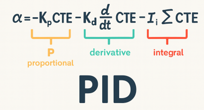
Let’s break it down:

Part 1 — P Control

Key Concepts:

Cross Track Error (CTE): The perpendicular distance between the vehicle and the desired path (reference trajectory). It tells us how far off course the vehicle is. A larger CTE means the car has drifted further from its desired path.

Imaging some naive approaches of control, might be like:

• Keeping the steering fixed (ineffective),
• Randomly adjusting toward the path (unreliable),
• Or — the ideal case — steering in proportion to the CTE.

Proportional Steering:

Proportional control means the further off you are, the stronger the correction. This approach allows the car to gradually reduce error and converge toward the path — smooth, intuitive, and effective.

In the process of correction, we introduce the gain constant τ (often called Kp in control systems) in the equation:

to control how aggressively or gently the system reacts to error.

Here is how to implement P-Control:

def run(robot, gain_tau, num_steps=100, forward_speed=1.0):
    # Store the trajectory of the robot
    x_path = []
    y_path = []

    for step in range(num_steps):
        # Cross-track error is the distance from the robot to the desired path (assumed to be y=0)
        cte = robot.y

        # Proportional control: steering angle is proportional to the negative of CTE
        # The negative sign helps steer the robot back toward the center line
        steering_angle = -gain_tau * cte

        # Move the robot with the computed steering and fixed forward speed
        robot.move(steering_angle, forward_speed)

        # Record current position for plotting or analysis
        x_path.append(robot.x)
        y_path.append(robot.y)

    return x_path, y_path

In reality, it overshoots the path due to momentum and delay. Over Time, the vehicle will keep zig-zagging back and forth around the desired trajectory. This happens because proportional correction always lags slightly behind the actual error.

Therefore, a P-Controller alone is simple but insufficient for perfect path tracking. It reduces error, but causes oscillation (due to overcorrection). Without damping (D-term) or bias correction (I-term), it leads to marginally stable behavior — not great for smooth control.

Part 2 — PD Control

PD Controller — Proportional-Derivative Control — an improvement over the basic P-controller.

Control Equation:

What’s New in PD Control?

• Proportional term: Still reacts to the size of the error — corrects based on how far off the robot is.
• Derivative term: Reacts to the rate of change — adds anticipation. If the error is decreasing quickly, it eases off the correction.

Why Add the Derivative Term?

• A P-controller alone tends to overshoot and oscillate.
• The D-term damps this oscillation, leading to: faster convergence, smoother motion and less zig-zagging.

PD Control can be implemented as:

def run(robot, proportional_gain, derivative_gain, num_steps=100, forward_speed=1.0):
    # Lists to store the trajectory of the robot
    x_path = []
    y_path = []

    # Initialize the previous cross-track error (CTE)
    previous_cte = robot.y

    for step in range(num_steps):
        # Current cross-track error: how far the robot is from the reference path (assumed to be y=0)
        current_cte = robot.y

        # Derivative of CTE: how quickly the error is changing (rate of error)
        diff_cte = current_cte - previous_cte

        # PD control law: steering is based on current error and how fast it's changing
        steering = -proportional_gain * current_cte - derivative_gain * diff_cte

        # Move the robot using the computed steering and forward speed
        robot.move(steering, forward_speed)

        # Store trajectory
        x_path.append(robot.x)
        y_path.append(robot.y)

        # Update previous error for next iteration
        previous_cte = current_cte

    return x_path, y_path

The PD controller corrects based on how far you are and how fast you’re approaching or moving away from the path — like having both a steering wheel and a brake.

🔧 Why PD is Not Enough

1. It can’t eliminate steady-state error (bias)

Imagine a car that consistently drifts to the right due to a misaligned steering wheel, or a drone that always gets pushed by a steady wind. These are constant biases.

• Proportional (P): Will steer to correct the error, but eventually settles with some small error.
• Derivative (D): Reacts to the change in error — so if the error becomes constant, D does nothing.

Result: The system might stabilize close to the reference, but never perfectly reaches it. This is called a steady-state error.

2. D term amplifies noise

• Since the D term looks at how fast the error is changing:

Even small measurement noise can cause large, spiky derivative values.

• This leads to jerky or unstable control, especially in real-world systems with imperfect sensors.

3. No memory of past errors

• PD reacts only to current and changing error.
• But what if your system has had persistent small errors over time?
• It has no “cumulative memory” — so it can’t compensate over time.

This is where the Integral (I) term helps — by accumulating past error and slowly pushing the system to fully zero it out.

Part 3 — PID Control

Full PID Control Formula:

The last part of the formula is I (Integral)

• Reacts to the sum of all past errors.
• Slowly eliminates persistent bias (like wind or sensor drift).
• Ensures you eventually reach the path.
• Acts like a long-term memory.

All together, the full PID can be implemented as:

def run(robot, Kp, Kd, Ki, num_steps=100, robot_speed=1.0):
    # Lists to record the robot's x and y positions over time
    x_trajectory = []
    y_trajectory = []

    # Initialize the integral of cross-track error (for the I term)
    total_cte = 0.0

    # Get the initial cross-track error (distance from path, y position)
    previous_cte = robot.y

    for step in range(num_steps):
        # Current cross-track error
        current_cte = robot.y

        # Derivative of cross-track error (change rate)
        delta_cte = current_cte - previous_cte

        # Accumulate cross-track error over time
        total_cte += current_cte

        # Update previous error for the next step
        previous_cte = current_cte

        # Calculate the steering angle using PID formula
        # Steering = -Kp * error - Kd * derivative - Ki * integral
        steer_angle = -Kp * current_cte \
                      - Kd * delta_cte \
                      - Ki * total_cte

        # Move the robot with calculated steering and constant speed
        robot.move(steer_angle, robot_speed)

        # Debug print for each step
        print(robot, steer_angle)

        # Store the current position
        x_trajectory.append(robot.x)
        y_trajectory.append(robot.y)

    return x_trajectory, y_trajectory

• Kp: Proportional gain — reacts to the present error.
• Kd: Derivative gain — reacts to the rate of change of the error (damping).
• Ki: Integral gain — reacts to the accumulated error (corrects long-term drift).
• cte: Cross-Track Error — how far the robot is from the desired path (assumed y = 0).
• robot.move(): Simulates the robot updating its position based on the steering angle.

Part 4 — How to find the best parameters

Now that we understand the full picture of PID control, a natural next question is: how do we choose the best parameters to make it work effectively?

This is where the Twiddle algorithm comes in — a simple but powerful heuristic optimization technique. Twiddle helps us automatically tune the PID controller parameters (Kp, Kd, and Ki) to minimize error and improve performance.

By systematically adjusting the values and observing the system’s response, Twiddle searches for the parameter combination that gives us the smoothest, most accurate control.

In the context of PID control, Twiddle adjusts the gains Kp (proportional), Kd (derivative), and Ki (integral) to minimize total error — for example, how far a car drifts from its target path. It can be implemented as:

def run_PID_controller(params):
    """
    Run the PID controller using the given parameters.
    Returns the total cross-track error over the trajectory.
    """
    Kp, Kd, Ki = params
    x_traj, y_traj = run(robot, Kp, Kd, Ki)

    # Calculate total squared cross-track error as a measure of performance
    total_error = sum([y**2 for y in y_traj])
    return total_error

def twiddle(tolerance=0.00001):
    """
    Uses the Twiddle algorithm to optimize PID parameters (Kp, Kd, Ki).
    """
    # Initial guesses for [Kp, Kd, Ki]
    pid_params = [0.0, 0.0, 0.0]

    # Initial adjustment amounts for each parameter
    param_deltas = [1.0, 1.0, 1.0]

    # Run with initial parameters and record the error
    best_error = run_PID_controller(pid_params)

    # Loop until the sum of parameter adjustments is small enough
    while sum(param_deltas) > tolerance:
        for i in range(len(pid_params)):
            # Try increasing the current parameter
            pid_params[i] += param_deltas[i]
            error = run_PID_controller(pid_params)

            if error < best_error:
                # Improvement found: accept and increase adjustment
                best_error = error
                param_deltas[i] *= 1.1
            else:
                # Try decreasing instead
                pid_params[i] -= 2 * param_deltas[i]
                error = run_PID_controller(pid_params)

                if error < best_error:
                    # Improvement found in the opposite direction
                    best_error = error
                    param_deltas[i] *= 1.1
                else:
                    # No improvement in either direction: revert and reduce adjustment
                    pid_params[i] += param_deltas[i]
                    param_deltas[i] *= 0.9

    return pid_params  # Return the best found [Kp, Kd, Ki]

Logic of Twiddle:

• Start with [Kp, Kd, Ki] = [0, 0, 0].
• Adjust each parameter slightly and evaluate the performance.
• If performance improves, increase that adjustment amount.
• If it gets worse, try the opposite direction, and if that fails too, reduce the adjustment.

Part 5 — Finding Smooth Path:

Now that we know how to control a robot using PID, the next question is: what exactly should it follow? In the real world, roads aren’t made up of sharp angles and jagged points. Before we even apply PID control, we often want to generate a smooth path — one that’s gentle, continuous, and safe for a robot or vehicle to follow.

This is where path smoothing comes in. Instead of commanding the robot to follow a rough, stepwise line, we refine the path into a curve that balances staying close to the original points while maintaining smooth transitions. Think of it like drawing a flowing ribbon through waypoints — reducing unnecessary steering effort and improving stability.

We first create a serial of y_i that are in the same location as x_i:

y_i = x_i, then we try to minimize the following terms:

• Error of original points with the smooth points: |x_i — y_i|
• Distance between th consecutive points: |y_i — y_i+1|

Path Smoothing Formula:

The alpa and beta controls if you want the path to be smoother or closer to the original path.

So, while PID control dynamically adjusts steering during movement, path smoothing adjusts the path itself beforehand to make it easier for the PID to follow.

from copy import deepcopy

def smooth(path, weight_data=0.5, weight_smooth=0.1, tolerance=0.000001):
    # Make a deep copy of path into newpath
    newpath = deepcopy(path)

    change = tolerance
    while change >= tolerance:
        change = 0.0
        for i in range(1, len(path) - 1):
            for j in range(len(path[0])):
                aux = newpath[i][j]
                newpath[i][j] += weight_data * (path[i][j] - newpath[i][j]) + \
                                 weight_smooth * (newpath[i-1][j] + newpath[i+1][j] - 2.0 * newpath[i][j])
                change += abs(aux - newpath[i][j])

    return newpath

How They Complement Each Other

• Smoothed path → fewer sharp turns → smaller errors → less oscillation in PID.
• PID controller → better able to follow the smoothed path without aggressive corrections.

In short: Path smoothing prepares the path, PID makes the robot follow it.

🛠️ Final Takeaway

First, smooth the path.

Then, use PID to follow it.

Tune it with Twiddle.

And your robot won’t zigzag — it’ll glide.

Reference:

Thrun, Sebastian. AI for Robotics. Available at: https://www.udacity.com/course/ai-for-robotics--cs373