The Evolution of GAN Architectures: PGGAN → StyleGAN → StyleGAN2

GAN architectures did not evolve randomly. Every major shift — from PGGAN to StyleGAN and eventually StyleGAN2 — happened because earlier ideas started creating problems they were never originally designed to solve. After implementing PGGAN myself, I realized something uncomfortable: what looked elegant on paper could quickly turn into an increasingly complex engineering problem in practice. In this article, we will follow the mathematical evolution of GAN architectures, understand why each transition happened, and explore why StyleGAN2 eventually moved beyond progressive growing.

Index

1. Progressive GAN (PGGAN): The Beginning of Progressive Learning

2. PGGAN Low Level Design Used By Me While Implementing it

3. Why PGGAN Failed for Me

4. StyleGAN: The Birth of Style-Based Generation

5. How StyleGAN Works

6. Why StyleGAN Felt Like a Major Shift From PGGAN

7. StyleGAN2: Rebuilding Image Generation

8. Conclusion

1. Progressive GAN (PGGAN): The Beginning of Progressive Learning

The Problem With Direct High-Resolution GAN Training

Before Progressive GAN (PGGAN), training GANs directly at high resolutions was extremely unstable. Asking a model to generate realistic 128×128, 256×256, or even larger images often resulted in noisy outputs, distorted structures, mode collapse, or complete training failure.

The challenge was deeper than image resolution itself.

Generating a realistic image requires learning multiple things simultaneously:

• Global structure (Where should the face exist?)
• Spatial relationships (Where should eyes, nose, and mouth be placed?)
• Fine textures (Hair, shadows, skin details)
• High-frequency realism (Sharp edges and local detail)

This created an optimization problem.

A generator that had not even learned where a face should exist was simultaneously expected to learn pixel-level realism.

In practice, this often made high-resolution GAN training unstable and difficult to scale.

Why PGGAN Was Revolutionary

In 2017, NVIDIA introduced Progressive GAN (PGGAN) with a surprisingly elegant idea:

What if GANs learned simple things first and difficult things later?

Instead of training directly at full resolution, PGGAN proposed progressive growing, where training begins from extremely small resolutions and gradually grows over time:

4×4 → 8×8 → 16×16 → 32×32 → 64×64 → 128×128

The intuition was simple.

At lower resolutions, the model focuses on coarse structure.

For example:

At 4×4, the model may only learn:

• facial position
• symmetry
• rough composition

At 16×16, it begins learning:

• eye regions
• nose placement
• facial proportions

At higher resolutions, it can refine:

• textures
• lighting
• realistic details

Instead of learning everything simultaneously, image generation becomes a staged learning process.

For its time, this idea was revolutionary because it made high-resolution GAN training significantly more practical.

However, as elegant as progressive learning sounded, it quietly introduced a new class of engineering and optimization challenges — some of which would only become obvious much later.

The Mathematics of Fade-In Training

One of the most important ideas introduced by PGGAN was fade-in training.

When moving from one resolution to another, PGGAN does not abruptly replace the old network with a new larger network. Instead, it gradually blends the newly added layers into the existing architecture.

For example, when transitioning from:

1616 → 3232

the generator initially relies almost entirely on the already-trained 16×16 pathway, while the newly introduced 32×32 block contributes very little.

Over time, this contribution slowly increases.

Mathematically, this blending process is controlled using an interpolation parameter called alpha (α):

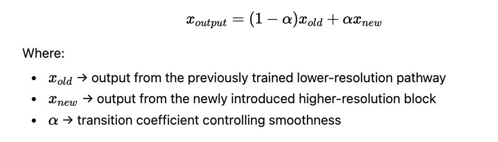
At

the model behaves entirely like the older resolution network.

At:

the newly introduced resolution completely takes over. The intuition behind fade-in training was simple:

Avoid shocking the network with sudden architectural changes.

Instead of forcing the generator to instantly learn higher — resolution details, PGGAN gradually transfers responsibility to the new layers.

In theory, this made training smoother and more stable.

However, it also introduced a subtle complication: the architecture itself changes while optimization is happening.

— a design decision that later became more important than it initially appeared.

Equalized Learning Rate, PixelNorm, and MiniBatch StdDev

PGGAN did not rely on progressive growing alone.

It also introduced several stabilization techniques that later influenced many GAN architectures:

Equalized Learning Rate (Equalized LR)

Instead of relying only on weight initialization to maintain stable activations, PGGAN dynamically rescales weights during training.

The goal was to stabilize feature magnitudes and improve optimization consistency.

Pixelwise Normalization (PixelNorm)

PixelNorm was introduced to normalize feature activations inside the generator.

This helped reduce activation magnitude instability and prevented features from growing uncontrollably during training.

MiniBatch Standard Deviation

MiniBatch StdDev was added near the discriminator output.

Its purpose was to help the discriminator detect:

low diversity mode collapse repetitive generations

Since I have already covered their mathematical intuition in detail in my previous article, I will not repeat the derivations here.

What matters for this discussion is that PGGAN was not merely a new training strategy.

It was an entire collection of architectural and optimization ideas designed to make high-resolution GAN training more practical.

What PGGAN Solved — And What It Quietly Introduced

Initially, PGGAN felt like an elegant engineering solution.

Instead of forcing a GAN to solve everything simultaneously, progressive learning allowed the model to gradually move from:

coarse structure → spatial arrangement → facial geometry → textures → realism

This solved an important problem: High-resolution GAN training became significantly more practical.

For its time, this was revolutionary.

However, progressive learning also introduced something subtle: Every resolution transition became its own optimization problem.

As the model grew:

4×4 → 8×8 → 16×16 → 32×32 → …

training dynamics changed.

New layers appeared.

Fade-in behavior changed optimization.

Different resolutions sometimes behaved differently.

Instead of training feeling like one continuous process, each stage could begin feeling like a partially new problem.

In hindsight, PGGAN reduced one major difficulty: direct high-resolution instability

but quietly introduced another: resolution-specific complexity

This tradeoff becomes especially important later when understanding why GAN architectures eventually evolved toward StyleGAN and ultimately StyleGAN2.

2. PGGAN Low Level Design Used By Me While Implementing it

I implemented a custom Progressive GAN using WGAN-GP for stable high-resolution face generation. The system progressively grows from 4×4 to 128×128 while combining Equalized Learning Rate, PixelNorm, Residual Connections, and MiniBatch Standard Deviation to improve training stability and feature learning.

Configuration I used:

Dataset: FFHQ

Image Resolutions: [4, 8, 16, 32, 64, 128]

Latent Dimension(Z_DIM): 128

Input Channels: 512

Image Channels: 3 (RGB)

Chunks Per Epoch: 4×4 → 5 chunks 8×8 → 4 chunks 16×16 → 3 chunks 32×32 → 3 chunks 64×64 → 1 chunk 128×128 → 1 chunk

Channel Configuration:

4*4 → 512

8*8 → 512

16*16 → 512

32*32 → 256

128*128 → 64

Generator Learning Rate Configuration:

4*4 → 2e-4

8*8 → 2e-4

16*16 → 2e-4

32*32 → 1e-4

64*64 → 1e^-4

128*128 → 1e-4

Critic Learning Rate Configuration:

4*4 → 2.5e-5

8*8 → 2.5e-5

16*16 → 2e-5

32*32 → 1e-4

64*64 → 1e-4

128*128 →1e-4

I need to manually tune critic or generator when required for a particular resolution.

Optimizer: Adam

Betas: (0.0, 0.99)

• β1 = 0.0 → disables momentum accumulation to avoid unstable GAN oscillations.
• β2= 0.99 → maintains smoother variance estimationfor stable adversarial optimization.

Gradient Penalty λ: 10

Progressive Epoch Schedule:

4*4 → 9 epochs

8*8 → 11 epochs

16*16 → 16 epochs

32*32 →30 epochs

64*64 → 40 epochs

128*128 → 50 epochs

Critic Iterations Per Stage:

4*4 → 1

8*8 → 2

16*16 →2

32*32 → 5

64*64 →5

128*128 →5

Residual Fade Epochs = 5

Residual Start Epochs = 5

Alpha Fade Epochs = 2

Stabilization Techniques Used:

• Equalized Learning Rate
• Pixel Norm
• Residual Connections
• MiniBatch Standard Deviation
• Progressive Growing
• Fade-in Transition
• WGAN-GP loss

Classes used in My PGGAN Implementation:

PixelNorm: A custom normalization layer in which I normalized feature magnitudes across channels to stabilize generator activations.

WSConv2D: A custom convolution layer in which I enforced Equalized Learning Rate for more stable GAN optimization instead of using standard nn.Conv2d

WSLinear: A custom fully connected (linear) layer in which I enforced Equalized Learning Rate instead of using standard nn.Linear

ConvBlock: A reusable convolution block combining WSConv2d →LeakyReLU →PixelNorm to avoid repeated code.

InitialGeneratorBlock:- A special generator block responsible for transforming latent noise vector into initial *44 feature maps.**

PGGANResidualBlock: A custom residual block in which I introduced skip connections for improved gradient flow in both generators and critic.

GeneratorBlock: A progressive generator module responsible for increasing spatial resolution through Upsampling → Residual Feature Learning during transitions from one resolution stage to the next (e.g., 4×4 → 8×8 → 16×16 → …).

CriticBlock: A progressive critic module responsible for Residual Feature Learning → Downsampling during transitions from higher to lower resolutions (e.g., 128×128 → 64×64 → 32×32).

MinibatchStdDev: A custom statistical layer in which I computed batch diversity and appended it as an extra feature map to help detect mode collapse.

ProgressiveGenerator: Main generator class controlling progressive growth, fade-in transitions, RGB conversion, and multi-resolution image synthesis.

ProgressiveCritic: Main critic class controlling progressive downsampling, fade-in transitions, and final real/fake scoring.

FinalCriticBlock: Final critic block responsible for minibatch statistics, final feature extraction, and critic score computation.

Important Class Methods

forward(): Defines forward computation logic for every neural network class.

fade_in(): Blends old and new resolutions during progressive growth.

train_progressive(): Controls full progressive training pipeline across all resolutions.

Implementation Design

Across my implementation, I followed a modular, stage-oriented system design architecture by combining multiple software design patterns to make the PGGAN system reusable, scalable, and easier to maintain.

At the lowest level, I followed a Wrapper (Decorator-like) pattern in WSConv2d and WSLinear by wrapping PyTorch’s native layers to enforce Equalized Learning Rate without modifying internal implementations.

I designed lightweight reusable components such as PixelNorm using a Utility pattern, while ConvBlock and PGGANResidualBlock followed Composite patterns, where I combined smaller reusable modules into standardized feature-learning pipelines with residual connections for stable training.

Higher-level components such as InitialGeneratorBlock, GeneratorBlock, CriticBlock, and FinalCriticBlock followed a Composite architecture, where reusable blocks were assembled progressively to support resolution growth.

At the full-system level, I designed ProgressiveGenerator and ProgressiveCritic using a Stage-Oriented Progressive Pipeline, enabling smooth resolution transitions through alpha fade-in.

Finally, I implemented train_single_epoch() and train_progressive() using a combination of Controller, Pipeline, and Template Method patterns, where I orchestrated checkpoint recovery, chunk-based data loading, progressive scheduling, critic-generator optimization, monitoring, and checkpoint persistence through a fixed but stage-adaptive training workflow.

Overall PGGAN Architecture

16*16 PGGAN Architecture

3. Why PGGAN Failed For Me

PGGAN did not fail for me because the original paper was fundamentally wrong or because progressive growing never works. For its time, it was one of the most important breakthroughs in stabilizing high-resolution GAN training. The real challenge, at least in my implementation experience, came from the practical instability introduced as training progressed across resolutions.

One of the most frustrating problems I encountered was persistent green-tinted image generation, where the generator would sometimes collapse toward unnatural green outputs despite training appearing numerically stable. What made this problem difficult to debug was that conventional indicators such as losses, gradients, and training progression often looked healthy, yet the generated images visually degraded. Instead of realistic facial structures, outputs became dominated by green color artifacts, indicating that the generator had learned an undesirable channel bias rather than balanced RGB feature generation.

This issue became especially noticeable during resolution transitions and fade-in stages. A configuration that appeared stable at lower resolutions such as 8×8 or 16×16 could suddenly behave differently after introducing a higher-resolution block. Since progressive growing continuously changes network depth, feature propagation, and optimization dynamics, every new resolution effectively altered the training behavior of the system. As a result, debugging often felt like solving a new optimization problem at every stage rather than continuing one stable training process.

Another challenge was that training behavior changed significantly across resolutions. Hyperparameters such as critic iterations, alpha scheduling, chunk selection, and residual transitions did not always generalize cleanly from one stage to another. A setup that worked at one resolution could unexpectedly fail at the next, producing artifacts, unstable colors, or poor feature quality. In my case, debugging became particularly difficult because the source of failure was often ambiguous — whether instability came from fade-in blending, critic imbalance, insufficient training at a specific stage, RGB channel bias, weight updates in newly introduced layers, or optimization mismatch.

Over time, I realized that PGGAN was not simply learning progressively higher-resolution images; it was progressively changing the optimization landscape itself. Instead of training one continuously improving model, the process often felt like repeatedly stabilizing a partially new system whenever the architecture grew.

4. StyleGAN: The Birth of Style-Based Generation

By the time, PGGAN had demonstrated that high-resolution image generation was possible, another problem slowly started becoming visible.

Generating realistic images did not necessarily mean generating controllable images.

Even when GANs produced visually convincing faces, the underlying latent space remained highly entangled.

A small change in the latent vector could unpredictably affect multiple visual properties at once.

For example:

changing what should ideally affect only:

hair style

might unexpectedly alter:

face shape lighting background facial expression

This lack of disentanglement made image generation difficult to control and harder to understand.

At the same time, progressive growing itself was beginning to reveal practical limitations.

Although PGGAN improved training stability, it also introduced resolution-specific complexity through staged learning and fade-in transitions.

The natural question became:

Could image generation be made more structured, controllable, and stable without depending so heavily on progressive learning?

This question ultimately led NVIDIA toward a new architectural direction: Style-based image generation.

Instead of feeding the latent vector directly into the generator and expecting it to learn everything implicitly, StyleGAN proposed something fundamentally different:

What if different visual attributes could be controlled at different levels of generation?

Rather than treating image synthesis as one monolithic process, StyleGAN attempted to separate high-level structure from fine visual details.

For example:

coarse styles could control:

• face shape
• pose
• overall composition

medium-level styles could influence:

• hairstyle
• facial features
• proportions

fine-level styles could refine:

• pores
• freckles
• hair strands
• texture

This shift was important because it changed the philosophy of image generation itself.

PGGAN primarily focused on How can we train high-resolution GANs

StyleGAN asked a different question: How can we make image generation more controllable and disentangled.

This marked the beginning of style-based generation, laying the foundation for one of the most influential families of generative models.

5. How StyleGAN Works

Why Traditional GAN Latent Space (Z) Was Entangled

Traditional GANs typically generate images using a simple idea:

A random latent vector is sampled from a probability distribution and directly passed into the generator

We generate a random vector, pass it through a neural network, and obtain an image.

However, NVIDIA observed an important limitation in traditional GANs:

The latent space Z was highly entangled.

Why should Z be entangled if it is sampled from a normal distribution where dimensions are independent?

So where does entanglement come from?

The answer lies not in the Gaussian distribution, but in how the generator learns to interpret Z.

Traditional GAN generators receive the latent vector directly and are expected to simultaneously learn:

• face geometry
• pose
• lighting
• hairstyle
• facial expression
• textures

using the same latent representations.

Since there is no explicit mechanism separating these visual properties, the generator learns complex nonlinear interactions between latent dimensions.

As a result, semantic information becomes mixed together.

For example, ideally we would want:

change hairstyle → hairstyle changes

But traditional GANs often behave like:

change hairstyle → hairstyle changes → face shape changes → lighting changes → background shifts

simultaneously

This phenomenon is called latent entanglement.

The problem was never that the Gaussian distribution itself was flawed. The problem was that: the generator was expected to organize meaningful semantic structure directly from an unstructured random latent space.

StyleGAN proposed a surprisingly elegant solution:

From Latent Space Z → Intermediate Latent Space W

Instead of directly feeding z, into the generator, StyleGAN introduces an intermediate transformation:

This creates a new latent space:

which becomes one of the most important innovations of StyleGAN.

Instead of forcing the generator to interpret a noisy and semantically mixed latent space directly, the mapping network learns a more structured representation before image synthesis begins.

Initially, adding another network may seem unnecessary.

Why increase complexity?

The answer lies in representation learning. The mapping network gradually reshapes the latent space into one where semantic image properties become easier to separate.

For example, directions in W-space may begin representing:

• face shape
• hairstyle
• age
• lighting
• expression

with far less interference between attributes.

This seemingly small architectural change had major consequences.

StyleGAN was no longer simply generating images.

It was the beginning to learn: how image attributes themselves should be organized.

The Mapping Network (MLP)

The mapping network in StyleGAN is mathematically simple but conceptually powerful.

It is implemented as a multilayer perceptron (MLP) consisting of multiple fully connected layers whose job is to learn:

In the original StyleGAN, this mapping network consists of 8 fully connected layers.

One question arises:

How can a simple MLP reorganize latent information into disentangled visual properties?

To understand this, we first need to understand what the MLP is mathematically doing.

A multilayer perceptron performs a sequence of nonlinear transformations:

This means the mapping network continuously warps the geometry of latent space through repeated non linear projections.

MLP learns a non linear mapping that “straightens” these directions.

How does the mapping network know what semantic properties should be separated?

There is no hard iteration count like:

10K iterations → disentangled

50K iterations → perfect W

because disentanglement is an emergent property, not an explicitly supervised target.

This mapping network is never told:

this neuron = hairstyle

this neuron = age

Instead, disentanglement gradually emerges during GAN optimization.

Measuring Disentanglement in W-space

1. Latent Traversal

Take a fixed latent vector w

and perturb one dimension at a time:

Then generate images.

Good disentanglement looks like:

change one direction → mostly one semantic property changes

2. Perceptual Path Length (PPL)

StyleGAN introduced a quantitative metric:

The idea: If W-space is disentangled and smooth, then:

small movement in latent space should produce smooth visual changes.

Mathematically:

Take two nearby latent points:

Measure image perceptual difference:

Normalize by latent distance:

Good W-space:

small latent movement → smooth visual change

Bad entanglement

small latent movement → chaotic image jump

Lower PPL generally indicates smoother disentanglement.

3. Linear Separability Tests

Researchers train simple classifiers on latent vectors.

Can a linear classifier separate:

• smiling vs non-smiling
• male vs female
• young vs old

inside W-space?

If able to classify, then semantic factors are more disentangled.

4. Visual Stability Across Layers

StyleGAN has coarse → medium → fine control.

If changing high-resolution styles only affects:

skin texture hair details

without changing:

face pose identity

that is evidence of disentanglement.

Disentanglement in StyleGAN is not a binary property — it is an optimization tendency. The mapping network gradually reorganizes latent geometry into a space where semantic factors become easier, not perfect, to separate.

Style Injection Through Adaptive Instance Normalization (AdaIN)

After learning a better latent representation:

StyleGAN introduces another important idea:

How should this latent information actually influence image generation?

Simply generating w is not enough.

The generator still needs a mechanism to decide:

which visual properties to modify

where to modify them.

at what scale to modify them

Traditional GANs mostly inject latent information only once, at the beginning of the generator.

StyleGAN changes this completely.

Instead of feeding latent information once

StyleGAN injects style information

into every generator layer

This happens through a mechanism called Adaptive Instance Normalisation (AdaIN)

Why Was AdaIN needed?

The key intuition behind AdaIN is simple.

Thinking progressively, different layers inside the generator control different semantic information.

Lower-resolution layers naturally influence:

• pose
• face geometry
• composition

Middle layers influence:

• eyes
• nose
• hairstyle
• facial proportions

Higher resolution layers refine

• skin texture
• pores
• hair strands
• fine details

So instead of giving generator one global vector and hoping it figures everything out.

StyleGAN asks:

What if every layer could receive its own style instructions?

AdaIN becomes the mechanism for delivering these instructions.

Step 1 — Instance Normalization

Suppose a feature map produced inside the generator is:

Before applying style, StyleGAN first normalizes activations channel-wise. For each feature channel:

Step 2 — Style Modulation

Now comes the important part.

The latent representation: w is transformed into two style parameters:

These values determine: how much each feature channel should be emphasized or suppressed.

Mathematically, an affine transformation is simply:

Affine Transformation is just a fully connected(linear) layer inside neural networks In StyleGAN.

You create one affine layer for every convolution layer in the generator.

Every feature starts from a normalized state.

Suppose affine layer produces:

Shape: 1024

StyleGAN simply splits this vector:

First half:

Second half:

Suppose channel 84 in w learned curly hair feature.

The splitting of y outputs into these two vectors is not decided dynamically. The split will be hardcoded by architecture design.

StyleGAN simply says:

First half → scaling

Second half → shifting

There is no learning about which part should scale or shift.

Then affine layer learns: If hairstyle should be stronger:

If hairstyle should reduce:

If feature activation should shift:

So affine layer is learning: How should each feature map be controlled for this specific image.

Step 3 — Adaptive Re-Scaling

After normalization, StyleGAN applies:

This equation is the heart of AdaIN.

Normalize first: Remove uncontrolled feature magnitude.

Then restyle: Reintroduce information using: through learned scaling and shifting. normalize → inject style → continue generation

AdaIN removes PixelNorm used in PGGAN because AdaIN already performs normalization. In PGGAN, PixelNorm was needed because feature magnitudes inside the generator could grow unpredictably. But in StyleGAN, every generator layer always performs Instance Normalisation. Feature maps get normalized channel-wise. Since normalization is already happening at every generator layer, PixelNorm becomes redundant.

Noise Injection: Adding Stochastic Details

Although AdaIN allows the generator to control meaningful semantic properties such as:

• face geometry
• pose
• hairstyle
• lighting
• expression

style information alone is not sufficient to generate realistic images. This is because not every visual detail in an image should be determined by latent semantics.

Some details are inherently stochastic, meaning they are naturally random and should vary even identity remains unchanged.

For example, two photographs of the same person may still differ in:

• individual hair strand placement
• skin pores
• micro skin texture
• tiny wrinkles
• freckles
• small lighting irregularities

These details do not define who the person is

Instead, they represent fine-scale randomness.

If StyleGAN tried to learn all these variations directly through the latent vector w, the generator would again begin mixing the semantic identity with random texture variation, making disentanglement harder.

StyleGAN therefore separates image generation into two responsibilities:

style (AdaIn): Controls what image should be.

Examples:

• identity
• face structure
• hairstyle
• expression
• pose

noise: controls small random visual details

Examples:

• hair strand randomness
• skin pores
• micro texture
• tiny freckles

Instead of forcing one latent representation to explain everything, StyleGAN explicitly separates semantic control from stochastic variation.

Step-1: Generate Spatial Noise

For every convolution layer inside the generator, StyleGAN injects a random noise map.

Step-2: Learnable Noise Strength

Simply adding raw noise would destabilize the training.

Instead, StyleGAN learns a trainable scaling coefficient for every feature channel

where i represents the feature channel.

This learnable parameter determines How much randomness should influence each feature map.

Initially

is randomly initialized (or near zero depending on implementation).

During training:

Generator loss backpropagates gradients.

If adding noise improves realism:

hair texture pores micro details

then gradient descent increases:

If noise harms image quality:

gradient pushes:

StyleGAN automatically learns how much randomness each feature channel should receive.

Step-3: Add Noise to Feature Maps

Suppose a feature map produced after convolution is: x

StyleGAN injects noise as:

is the random spatial noise map.

After this:

Noise Addition ↓ LeakyReLU ↓ Next Convolution Layer

training continues normally.

StyleGAN does not use noise to change image identity.

Instead, noise only introduces subtle visual randomness.

Without noise injection, generated images often appear:

overly smooth plastic-like artificial

With properly learned noise injection, StyleGAN produces:

natural hair strands skin micro-textures pores fine stochastic realism

This seemingly simple idea allowed StyleGAN to generate images that looked significantly more natural than earlier GAN architectures while preserving disentangled semantic control.

Style Mixing Regularization

After introducing AdaIN and layer-wise style control, another important problem emerged:

What prevents the generator from becoming overly dependent on one single latent representation?

Even though StyleGAN injects style into every layer, if all layers always receive the same latent vector, the network may still learn strong dependencies between layers.

Suppose one latent direction controls: hairstyle

Ideally we would want:

change hairstyle ↓ only hairstyle changes

But without additional constraints, the generator may begin learning hidden feature dependencies.

This phenomenon is called feature co-adaptation, where multiple generator layers become tightly coordinated and dependent on each other.

As a result: disentanglement weakens.

Changing one latent factor may unexpectedly modify several visual properties simultaneously.

To address this problem, StyleGAN introduced Style Mixing Regularization.

The idea is surprisingly simple:

Instead of always using one latent vector:

StyleGAN sometimes samples:

during training.

Rather than feeding the same style vector to every layer, StyleGAN randomly chooses a crossover point.

Example:

4×4 block → w1 8×8 block → w1 16×16 block → w2 32×32 block → w2

The crossover location changes randomly during training. This forces the generator to learn an important constraint:

Every layer must independently understand how to generate meaningful features.

A layer can no longer assume:

previous layers will always use the same latent code

because suddenly:

earlier layers → w1 later layers → w2

may appear

As a result, StyleGAN gradually learns:

coarse styles medium styles fine styles

more independently.

This improves disentanglement, because semantic factors become less entangled across resolutions and generator stages.

How NVIDIA Modified PGGAN Loss Function in StyleGAN

Although StyleGAN introduced major architectural innovations such as the mapping network, W-space, AdaIN, noise injection, and style mixing regularization, NVIDIA also made an important change that is often overlooked:

They modified the GAN training objective itself.

Since StyleGAN was built directly on top of PGGAN, one might expect it to continue using the same training loss. However, NVIDIA realized that improving architecture alone was not sufficient; training stability also depended heavily on the optimization objective.

In PGGAN, training primarily relied on Wasserstein GAN with Gradient Penalty (WGAN-GP). The critic loss was designed to estimate Wasserstein distance while enforcing Lipschitz continuity through a computationally expensive gradient penalty term.

WGAN-GP critic objective:

Generator objective:

Although WGAN-GP improved training stability compared to earlier GAN formulations, it introduced practical limitations. The gradient penalty term was computationally expensive, required additional gradient computations on interpolated samples, and often slowed training significantly at higher resolutions.

To address this, StyleGAN moved toward a non-saturating logistic loss with R1 regularization, which simplified optimization while preserving stability.

R1 Regularization is a discriminator regularization technique introduced to stabilize training without using gradient penality like WGAN-GP.

The discriminator or the critic should not react too sharply to tiny changes in real images.

If the discriminator becomes too aggressive, generator training becomes unstable because gradients become noisy or explode.

So instead of penalizing gradients on interpolated images like WGAN-GP:

real ↔ fake interpolation

Mathematically:

R1 Regularization only penalizes real image gradients. No interpolation. No Lipschitz constraint. Much cheaper computationally

Unlike WGAN-GP, which directly uses raw critic scores:

D(real) D(fake)

StyleGAN applies a smooth nonlinear transformation using:

commonly called the softplus function.

Instead of directly optimizing critic outputs, NVIDIA introduced exponential and logarithmic transformations over critic scores to make optimization smoother and gradients more stable.

SoftPlus helps prevent unstable optimization behavior caused by extremely large positive or negative discriminator outputs, producing smoother gradients during training.

StyleGAN discriminator objective:

StyleGAN generator objective:

This change brought several practical advantages:

faster training lower computational overhead simpler optimization better discriminator stability

6. Why StyleGAN Felt Like a Major Shift From PGGAN

After implementing and debugging PGGAN, StyleGAN felt less like a minor architectural improvement and more like a fundamental shift in how image generation was approached. In PGGAN, the generator receives a single latent vector at the beginning and is expected to learn everything — identity, pose, lighting, hairstyle, and fine textures — from the same entangled representation. This often made generation difficult to interpret and unstable to control, where changing one latent direction could unintentionally alter multiple visual properties simultaneously. StyleGAN addressed this limitation by introducing a mapping network, W-space, layer-wise style injection through AdaIN, noise injection, and style mixing regularization, which gradually separated semantic structure from stochastic detail. Instead of treating generation as one monolithic black-box transformation, StyleGAN organized image synthesis hierarchically — early layers controlling coarse structure, middle layers controlling facial attributes, and higher-resolution layers refining fine textures. From an implementation perspective, this made image generation feel more interpretable, semantically controllable, and significantly easier to reason about compared to the highly entangled behavior often experienced during PGGAN training.

7. StyleGAN2: Rebuilding Image Generation

Why StyleGAN1 Was Still Not Enough

StyleGAN represented a major breakthrough in image generation. Compared to PGGAN, it introduced W-space disentanglement, layer-wise style control through AdaIN, noise injection, and style mixing regularization, making image synthesis significantly more controllable and interpretable. For the first time, different generator layers could influence different semantic aspects of an image, allowing meaningful control over coarse structure, facial attributes, and fine textures.

However, despite these improvements, NVIDIA soon realized that StyleGAN1 still suffered from several important limitations that prevented it from being the final solution for high-quality image generation.

One of the most noticeable problems was the presence of characteristic visual artifacts, particularly the well-known blob-like or water-droplet artifacts that occasionally appeared in generated images. Although StyleGAN images looked highly realistic initially, closer inspection sometimes revealed strange texture inconsistencies, repetitive patterns, or localized distortions that reduced realism. These artifacts suggested that image quality had improved significantly, but the internal signal processing of the generator was still not fully stable.

Another major issue came from Adaptive Instance Normalization (AdaIN) itself. Although AdaIN enabled powerful style control, repeatedly normalizing feature maps at every layer sometimes disrupted important signal statistics. Since StyleGAN constantly normalized and restyled activations, certain feature magnitudes became artificially manipulated, occasionally producing unrealistic texture behavior and subtle structural inconsistencies. In other words:

AdaIN improved controllability, but sometimes at the cost of signal fidelity.

Training behavior could still change significantly when moving between resolutions, meaning image generation remained dependent on carefully tuned progressive schedules.

Another limitation was that latent disentanglement was still imperfect. Although W-space dramatically improved semantic separation compared to traditional GANs, latent factors were not completely independent. Certain latent directions could still unintentionally affect multiple visual properties simultaneously.

Over time, NVIDIA realized an important lesson:

Improving semantic controllability alone was not enough.

The architecture also needed:

better signal preservation artifact reduction simpler training dynamics more stable feature propagation

This realization ultimately led to the development of: StyleGAN2 which was not a complete redesign of StyleGAN, but rather a careful rethinking of the hidden weaknesses introduced by StyleGAN1 itself.

What NVIDIA Realized About AdaIN

Although Adaptive Instance Normalization (AdaIN) became one of the most celebrated innovations of StyleGAN, NVIDIA eventually realised that it was also responsible for several hidden problems inside the generator.

Initially, AdaIN seemed like an elegant solution. It allowed StyleGAN to inject style information into every generator layer by first normalizing feature activations and then restyling them through learned scaling and shifting parameters. This made semantic control significantly better than earlier GAN architectures.

The intuition behind AdaIN was powerful:

normalize features ↓ remove uncontrolled statistics ↓ inject desired style ↓ continue generation

However, NVIDIA later discovered an important problem: AdaIN was repeatedly overriding feature statistics at every layer.

Every time AdaIN was applied, the generator first normalized activations:

mean → reset variance → reset

and then reintroduced style through scaling and shifting.

Although this improved style controllability, it unintentionally disrupted important information already learned inside feature maps.

The generator was constantly destroying and rebuilding activation statistics.

This created an unstable signal propagation process.

Instead of preserving naturally evolving feature distributions, StyleGAN repeatedly forced features into normalized states and then restyled them again.

Over many layers, this sometimes introduced:

texture inconsistencies unnatural feature amplification artifact formation signal distortion

One of the clearest consequences became the well-known:

water droplet blob-like artifacts

observed in some StyleGAN-generated images.

NVIDIA realized something subtle but important: The problem was not style injection itself. The problem was where style was being injected.

Instead of modifying feature activations after convolution, perhaps style should directly influence the convolution operation itself.

This realization became the foundation of one of the biggest architectural changes in StyleGAN2: Removing AdaIN and replacing it with Weight Modulation where style no longer manipulates feature maps directly, but instead controls the convolution weights themselves.

Removing AdaIN: From Style Injection to Weight Modulation

StyleGAN2 injects styles into weights using a technique called: Weight Modulation

The key idea is Instead of modifying feature maps after convolution (AdaIN), StyleGAN modifies convolution weights before convolution happens.

Suppose in a normal convolution layer:

Weights are:

Feature input:

Normal convolution:

where:

same weights for every image

Just like StyleGAN1:

Latent vector: z passes through the MLP mapping network:

No change here.

For every convolution layer:

StyleGAN2 still uses:

one affine layer per convolution layer

But now affine output is:

instead of:

Example:

If:

Affine produces:

Meaning: one style coefficient per input channel

Instead of applying style to feature maps:

StyleGAN2 scales weights channel-wise.

Original weights:

become:

For every input channel:

multiply entire kernel by style coefficient

The latent style now influences how convolution kernels behave before feature generation begins.

This change may seem subtle, but it fundamentally changed how signal propagation worked inside the generator.

By moving style control into convolution itself, StyleGAN2 preserved feature statistics more naturally, reduced artifacts, and improved signal consistency across layers.

In many ways, this became one of the most important architectural redesigns separating StyleGAN2 from StyleGAN1.

Weight Demodulation

Although weight modulation solved many of the problems introduced by AdaIN, NVIDIA soon discovered that it unintentionally created a new issue.

Modulating convolution weights could accidentally amplify feature magnitudes too much.

The affine layer produces style coefficients: s

which directly scale convolution weights:

This allows style to influence:

• which channels become stronger
• which channels become weaker

However, NVIDIA realized an important consequence.Suppose style coefficients become large: Then certain convolution channels suddenly become heavily amplified. As convolution progresses across layers, this can lead to:

uneven feature magnitudes activation explosion channel imbalance unstable signal propagation

Some feature channels started dominating too much.

Instead of balanced feature learning, the generator could unintentionally overemphasize certain channels, causing inconsistencies in generated textures and image quality.

NVIDIA therefore introduced another important idea: Weight Demodulation

After modulating weights, normalize them again so that no channel becomes excessively dominant.

Modulate weights ↓ control amplification ↓ perform convolution

Mathematically, StyleGAN2 computes a normalization factor for each output channel.

Suppose modulated weights are:

Demodulation computes:

Then weights are normalized:

Every output channel is automatically rescaled to maintain stable signal magnitude.

The full StyleGAN2 flow becomes:

Affine Layer ↓ Style Coefficients ↓ Weight Modulation ↓ Weight Demodulation ↓ Convolution ↓ Feature Generation

Weight Modulation asks which features should become stronger?

Weight Demodulation asks how to prevent those features from becoming too dominant?

Together, modulation and demodulation created a much more stable feature generation process than AdaIN.

Instead of repeatedly destroying feature statistics through normalization, StyleGAN2 preserved signal propagation naturally while still allowing powerful style control.

Removing Progressive Growing

One of the most important architectural decisions in StyleGAN2 was the removal of progressive growing, even though progressive training had originally been one of the core ideas behind PGGAN and early StyleGAN. NVIDIA realized that while progressive growing initially helped stabilize high-resolution GAN training, it also introduced many hidden optimization and engineering problems. Every time a new resolution layer was added, the training dynamics changed, feature propagation shifted, and fade-in transitions introduced additional instability. In practice, this often made training feel like repeatedly adapting to partially different optimization problems at every stage of growth rather than training one continuously stable model. This closely matched many of the issues I also experienced during my own PGGAN implementation.

However, it is important to clarify what “removing progressive growing” actually means in StyleGAN2. StyleGAN2 did not completely remove the multi-resolution architecture itself. The network still contains hierarchical resolution blocks such as 4×4, 8×8, 16×16, 32×32, and so on. The difference is that these layers are no longer introduced progressively during training. Instead of dynamically creating higher-resolution blocks at runtime and blending them through fade-in transitions, StyleGAN2 trains the entire architecture from the beginning. All resolution blocks are present from the start, and training occurs simultaneously across the full network. In other words, StyleGAN2 removed progressive training, not the multi-scale hierarchical structure of the generator and discriminator. This eliminated fade-in instability while preserving the benefits of coarse-to-fine feature learning across resolutions.

Surprisingly, improvements introduced in StyleGAN2 — particularly:

weight modulation weight demodulation better signal propagation improved regularization

had already stabilized training enough that progressive growing was no longer necessary.

Path Length Regularization

Even after removing AdaIN artifacts and abandoning progressive growing, NVIDIA realized another subtle problem still remained inside StyleGAN2: Latent space transformations were not always smooth or predictable.

Ideally, when we slightly modify a latent vector: w the generated image should also change smoothly and proportionally.

For example:

A small movement in latent space should produce:

slightly different hairstyle slightly different expression small pose variation

Instead of

sudden facial distortion identity jump large unexpected visual changes

However, NVIDIA observed that generator sensitivity across latent space was often inconsistent.

Some latent directions caused: tiny visual changes while others produced massive image transformations.

This created an uneven latent geometry. Equal movement in latent space did not always produce equal movement in image space.

NVIDIA wanted StyleGAN2 to learn a smoother relationship:

small latent movement ↓ small image change

large latent movement ↓ large image change

This led to the introduction of: Path Length Regularization

Instead of only focusing on realism, NVIDIA also wanted latent traversal to become:

smooth predictable stable semantically meaningful

Path length regularization encourages: similar latent movement → similar image movement

Jacobian tells: How much output changes when input changes

For generator:

Jacobian:

Meaning:

how sensitive image pixels are to latent changes

If Jacobian magnitude is: very large: generator too sensitive

very small: generator barely reacts

NVIDIA wanted: consistent sensitivity

But image output is huge:

1024×1024×3 pixels

Direct Jacobian computation is expensive.

So they used a trick. Instead of checking all directions: They sample a random direction: y in image space. Then compute.

This tells: How strongly image changes along a random direction when moving in latent space?

Then measure its magnitude:

Meaning: how strong latent movement feels

NVIDIA says: We want this sensitivity to remain near some average target.

Suppose desired average sensitivity:

Then penalize deviation:

too sensitive → penalty too insensitive → penalty

This becomes:

Loss Function in StyleGAN2

Although StyleGAN2 is often remembered for architectural improvements such as weight modulation, weight demodulation, and removal of progressive growing, NVIDIA also introduced an important training modification:

They improved the generator objective by introducing Path Length Regularization.

Unlike PGGAN, which used WGAN-GP, and StyleGAN1, which used non-saturating logistic loss with R1 regularization, StyleGAN2 retained the StyleGAN1 optimization framework while adding an additional regularization term focused on improving latent-space smoothness.

The core adversarial objective remained similar to StyleGAN1.

Discriminator Loss

StyleGAN2 continued using:

• Non-saturating logistic loss
• R1 regularization

Discriminator objective:

where:

• first term penalizes fake images being classified as real
• second term rewards correct real image classification
• third term represents R1 regularization, stabilizing discriminator gradients on real images

Thus, discriminator training philosophy remained largely unchanged from StyleGAN1. The major modification came inside the generator objective. In StyleGAN1, the generator only optimized for: image realism

However, NVIDIA realized that realism alone was insufficient.

They also wanted:

smooth latent traversal predictable image edits stable semantic transitions consistent generator sensitivity

This led to the introduction of: Path Length Regularization

which acts as a generator-side gradient regularization term.

Path length objective:

This term encourages: equal movement in latent space → proportional movement in image space

Finally, StyleGAN2 generator loss becomes:

This means StyleGAN2 no longer optimized only for: realistic images

It simultaneously optimized for:

smooth latent geometry stable interpolation semantic consistency better controllability

StyleGAN2 was not only learning to generate realistic images, but also learning how image changes should behave in latent space.

Residual Connections and Skip Architecture in StyleGAN2

Although StyleGAN2 is most commonly discussed through innovations such as weight modulation, weight demodulation, removal of AdaIN, and Path Length Regularization, NVIDIA also redesigned how information flows through the generator and discriminator using skip connections and residual learning principles.

As GAN architectures became deeper and higher-resolution image synthesis became more demanding, training stability increasingly depended on reliable gradient propagation and stable feature preservation. Sequential convolutional layers alone can sometimes struggle because information gradually weakens as it passes through many transformations. This creates optimization difficulties and unstable feature learning.

To address this, StyleGAN2 adopted two different architectural strategies:

Generator → Skip Architecture Discriminator → Residual Architecture

Skip Architecture in the Generator

Unlike PGGAN and early StyleGAN, where image synthesis primarily depended on the final high-resolution feature maps, StyleGAN2 introduced a skip generator architecture using multiple ToRGB layers.

Instead of generating RGB only at the final layer, intermediate generator blocks directly contribute to the final image.

For example:

At every resolution, a ToRGB layer converts feature maps into RGB space. These intermediate RGB outputs are upsampled and accumulated progressively into the final image.

The intuition behind this design is important.

Lower-resolution layers already learn meaningful coarse semantic information such as:

• face structure
• identity
• pose
• composition

Higher-resolution layers mainly refine:

• skin texture
• pores
• hair strands
• fine stochastic realism

Instead of forcing high-resolution layers to reconstruct everything again, StyleGAN2 allows earlier semantic information to directly influence the final image through skip pathways.

This improved:

• signal preservation
• gradient flow
• semantic consistency
• high-resolution stability

Residual Architecture in the Discriminator

While the generator primarily uses skip connections, the discriminator more explicitly follows a ResNet-style residual architecture.

StyleGAN2 supports residual downsampling blocks where information bypasses convolutional transformations through shortcut paths.

Conceptually:

Input ├── Main Path: │ Conv → LeakyReLU │ Conv → Downsample │ └── Skip Path: 1×1 Conv → Downsample

Output: (Main Path + Skip Path) / √2

Instead of learning entirely new feature transformations at every stage, the discriminator learns residual corrections over existing features.

The skip pathway preserves information, while the main pathway refines it. The normalization factor:

helps stabilize feature magnitudes after feature fusion.

This residual design improved:

• gradient propagation
• optimization stability
• deep feature learning
• training robustness at higher resolutions

In practice, StyleGAN2 primarily uses skip connections in the generator and residual connections in the discriminator, although NVIDIA also supported residual-style generator variants in implementation. Together, these architectural improvements helped StyleGAN2 achieve cleaner image synthesis, stronger signal preservation, and more stable optimization than earlier GAN architectures.

8. Conclusion

The evolution from PGGAN → StyleGAN → StyleGAN2 was not a sequence of random architectural upgrades. Each transition happened because earlier solutions eventually exposed new limitations that demanded better design choices. PGGAN solved one of the biggest challenges of its time by making high-resolution GAN training practical through progressive growing, fade-in transitions, and stabilization techniques such as Equalized Learning Rate, PixelNorm, and MiniBatch Standard Deviation. However, during implementation, it also revealed an uncomfortable reality: training stability often became resolution-dependent, introducing engineering complexity, debugging overhead, and unpredictable behavior across stages. In my own implementation, this became especially visible through issues such as green-tinted image collapse, unstable transitions, and stage-specific tuning requirements.

StyleGAN represented a philosophical shift. Instead of asking only:

How can we train high-resolution GANs?

it asked:

How can image generation become controllable and disentangled?

Through W-space, mapping networks, AdaIN, noise injection, and style mixing regularization, StyleGAN introduced a more structured view of image synthesis where different layers learned different visual responsibilities. Image generation became significantly more interpretable and semantically controllable. Yet even StyleGAN was not perfect. AdaIN introduced hidden signal distortions, artifacts emerged, and progressive growing continued carrying optimization complexity.

StyleGAN2 therefore did not simply improve StyleGAN — it carefully rethought many of its hidden weaknesses. By replacing AdaIN with weight modulation and demodulation, removing progressive growing, and introducing Path Length Regularization, NVIDIA shifted attention toward stable signal propagation, artifact reduction, and smooth latent geometry. Image generation was no longer optimized only for realism, but also for predictability, controllability, and meaningful semantic transitions in latent space.

For me, one of the biggest lessons from this evolution was realizing that breakthroughs in deep learning often emerge not because earlier ideas completely fail, but because they eventually expose the next bottleneck. PGGAN made high-resolution generation possible. StyleGAN made generation controllable. StyleGAN2 made it cleaner, smoother, and more stable. Understanding this progression changed how I think about model design itself:

Every elegant idea eventually creates new constraints — and progress often begins by understanding those hidden limitations deeply enough to redesign the system around them.