How I Built a Self-Scaling AI Inference Cluster from Scratch

From a single model running on a laptop to a distributed system serving hundreds of users — and what I learned along the way.

I started with a simple question: what actually happens when you try to serve an AI model to a thousand people at once?

The answer turned out to involve five completely different fields of computer science — memory management, distributed routing, task scheduling, feedback control theory, and yes, some linear algebra. Each one solved a real bottleneck I hit along the way.

This post is a tour of those five ideas. I won’t go deep on any of them — for that, I’ve linked the full technical writeup at the end. What I want to give you here is the intuition behind each piece, and why it matters.

The starting point: 17 tokens per second

A language model generates text one token at a time. Each token requires a full mathematical pass through the model — billions of floating point operations. On a laptop, running a small 0.5B parameter model, I was getting about 17 tokens per second on a cold start. Warmed up, around 54.

That’s fine for one person. The moment four people try to use it simultaneously, the naive approach produces 31 tokens per second total — about the same as one person alone. All that concurrency, no actual benefit.

The gap between 31 tok/s and 397 tok/s (what I ended up with) is the story of the next five ideas.

Part 1: The Memory Problem Nobody Talks About

The KV Cache — and why naive memory allocation wastes 60–80% of your GPU

When a model generates token #50 in a response, it needs the computed “key” and “value” vectors for all 49 previous tokens. Without a cache, it recomputes them from scratch every single time. That means generating a 1000-token response costs roughly a million times more computation than it needs to.

The fix — the KV cache — stores those vectors and reuses them. Simple idea. But it creates a new problem: memory management.

The naive approach is to allocate one big contiguous memory block per conversation. This seems fine until you think about what happens when conversations start and end at unpredictable times. The freed blocks scatter across memory like holes in Swiss cheese. A new conversation needs a 200-slot block but can only find gaps of 10 here, 15 there. You have 40% of memory free but can’t use it. This is fragmentation.

KV Cache Block Allocation — fixed-size blocks, free list, prefix sharing, and copy-on-write

The solution is borrowed directly from operating systems: paging. Instead of one block per conversation, divide all memory into small equal-sized blocks (16 tokens each). Every block is identical and interchangeable. A conversation gets whatever blocks are free — they don’t need to be adjacent. A block table keeps track of which blocks belong to which conversation.

Two more tricks make this powerful:

Prefix caching. If every API request starts with the same 2,000-token system prompt, you’re computing those vectors a hundred times. Instead, let multiple conversations share the same physical memory blocks for that prefix. Use a reference counter to track how many conversations are using each block.

Copy-on-write. If two conversations share a block and one needs to write new data into it, don’t corrupt the shared block — allocate a private copy first, then write. This is exactly how Unix handles the fork() system call.

The research paper behind vLLM measured fragmentation wasting 60–80% of GPU memory with the naive approach. Blocks bring that to under 4%.

Part 2: Serving Many People at Once

The Scheduler — how batching turned 31 tok/s into 397 tok/s

Here’s the ugly truth about Python threads: they don’t actually run in parallel for CPU-bound work. Python’s Global Interpreter Lock (GIL) means only one thread executes Python code at any moment. Four HTTP handler threads each calling model.generate() don't run four times as fast. They take turns, each waiting for the others, producing roughly the same speed as one.

The scheduler routes around this with two ideas.

One worker thread owns the model. HTTP handler threads don’t call the model at all. They create a request, drop it into a priority queue, and wait. A single background thread pulls requests from the queue and runs the model. No GIL contention — only one thread ever touches the model.

Batching. After the first request arrives, the worker thread waits up to 20ms for more. If three more arrive in that window, it processes all four together in a single model call. Why does this help so much?

A neural network’s forward pass is dominated by matrix multiplications. Processing one sequence uses a fraction of the GPU’s capacity. Processing eight sequences stacks them into a larger matrix and uses the full capacity. The arithmetic is eight times as much, but the overhead — kernel setup, memory transfers, Python interpretation — is paid once for the whole batch. Throughput multiplies.

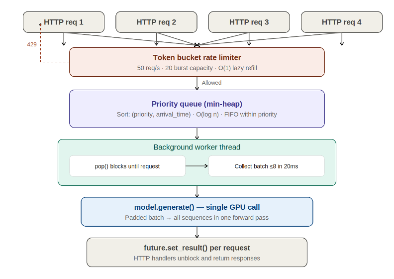
Scheduler Request Flow — rate limiting, priority queue, batching, and future-based dispatch

The priority queue is a heap — a data structure that always keeps the most urgent request at the top, with O(log n) insertion and extraction. Two requests at the same priority level are served in arrival order (FIFO). A token bucket rate limiter sits in front, allowing short bursts (a bucket that fills up over time) while rejecting sustained floods.

Result: 31 tok/s with naive threading → 397 tok/s with the scheduler. Same hardware. No other changes.

Part 3: Routing Across Multiple Machines

Consistent Hashing — adding a second worker without breaking everyone’s cache

At some point, one machine isn’t enough. You add a second server. Now every incoming request needs to be directed to one of them. Simple, right? Round-robin — alternate between workers — distributes load evenly.

Except it breaks your cache.

Each worker has been building a KV cache for the conversations it’s been handling. If conversation #42 has been talking to worker-1 for ten messages, worker-1 has ten messages’ worth of cached vectors. When message eleven arrives, round-robin sends it to worker-2. Worker-2 has no cache. It recomputes everything from scratch. The cache on worker-1 is wasted.

You need session affinity — the same conversation always goes to the same worker. The naive approach: hash(session_id) % number_of_workers. This works fine until you add or remove a worker. With 3 workers, session #42 routes to worker hash(42) % 3 = 0. Add a fourth worker: hash(42) % 4 = 2. Session #42 now routes to the wrong worker. And this doesn't just affect session #42 — ~75% of all active sessions remap simultaneously when you add one worker.

: Consistent Hash Ring — virtual nodes, minimal remapping, and failover routing

Consistent hashing solves this by placing both workers and sessions on a ring — a circle with 4 billion positions. Each session hashes to a position and goes to the nearest worker clockwise. Add a new worker? It only “captures” sessions in its immediate arc. On average, only 1/n of sessions remap when you add a worker to an n-worker cluster. With 3 workers → 4 workers, that’s 25% instead of 75%.

But random placement on the ring means load might be uneven — one worker could own a huge arc and handle 90% of traffic. The fix: virtual nodes. Each physical worker claims 150 positions scattered around the ring instead of one. By the law of large numbers, this produces near-uniform distribution (measured at 52% / 48% in my test with two workers).

A heartbeat monitor polls each worker’s /health endpoint. Three consecutive failures → declare the worker down and remove it from the ring. Two consecutive successes → add it back. This asymmetry (3 to go down, 2 to recover) creates inertia and prevents a flapping worker from causing constant disruption.

Part 4: Knowing When You’re Struggling

The PID Controller — the same mechanism as your home thermostat

You now have a multi-worker cluster that distributes load intelligently. But how does it know when to add another worker? And how does it avoid oscillating — adding one, removing one, adding one again?

The answer is a PID controller. You interact with one every day: your home thermostat.

A simple on/off thermostat overshoots. It heats the room past the target, turns off, cools below the target, turns on again. It hunts. A smarter thermostat considers three things simultaneously:

• How far am I from the target right now? → Proportional term (P)
• How long have I been off target, and by how much? → Integral term (I)
• Is the situation improving or worsening, and how fast? → Derivative term (D)

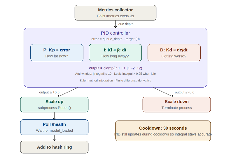
PID Autoscaler Control Loop proportional, integral, and derivative terms driving scale decisions

For the autoscaler: the “temperature” is queue depth (requests waiting). The “target” is zero. The control output is how many workers to add or remove.

The P term reacts to the current queue: queue=8, add workers. The I term accumulates history: if the queue has been slightly elevated for a long time, push harder. This eliminates steady-state offset — without it, the controller would settle at a slightly non-zero queue depth because it needs some error to produce any output. The D term anticipates: if the queue is dropping fast, back off before you overshoot.

Two practical additions: anti-windup prevents the integral from accumulating beyond useful limits when the system is saturated (otherwise it causes over-correction after load subsides). A leak term gently decays the integral toward zero during idle periods, so a past load spike doesn’t bias the controller indefinitely.

During the burst test (50 simultaneous requests), the controller fired a scale-up event at queue depth=6, output=+2.0. The integral decayed cleanly after the flood ended. Zero errors across all 50 requests.

Part 5: Watching the System Watch Itself

Metrics, Anomaly Detection, and the Full Loop

The final piece is observability — the system monitoring itself and surfacing problems before users notice them.

Every worker exposes a /metrics endpoint. A collector polls them every 3 seconds and aggregates: queue depth across all workers (fed to the PID controller), latency distribution (mean, p95, p99), and cache utilisation.

For anomaly detection, the system uses a z-score: for each new latency measurement, compute how many standard deviations it is from the recent rolling average. A z-score above 3 means the value is more than 3 standard deviations from normal — which happens by chance only 3 times in 1,000 measurements under normal conditions. No manual threshold needed; the system calibrates itself from real traffic.

End-to-End System Architecture — all five layers connected

When an autoscaled worker starts, it doesn’t immediately receive traffic. The system waits for the worker to report model_loaded: true in its health check before adding it to the hash ring. Loading the model takes 60-90 seconds on a development machine — routing traffic there before it's ready would cause immediate failures for every user unlucky enough to land on it.

The Numbers

Scenario Throughput Baseline, cold start, sequential 17 tok/s Baseline, warmed up, sequential 54 tok/s Naive 4-thread concurrency 31 tok/s With scheduler + batching 210 tok/s Full cluster, burst of 50 requests 397 tok/s

Router overhead: ~3ms per request. Session affinity: 100% (same conversation, same worker, every time). Scale-up event: fired correctly at queue depth=6. Errors across 50 concurrent requests: 0.

What’s Next

A few honest limitations: the custom memory manager isn’t yet wired into the model’s actual forward pass (it’s the right infrastructure, but needs custom CUDA kernels to intercept tensors at each layer — the same challenge vLLM solved). The cluster runs on one physical machine using different ports. There’s no durable request queue surviving a router crash.

These are the natural next steps — and they’re each a chapter in their own right.

Full technical deep-dive, code walkthrough, and all the math: github.com/shashanka300/Distributed-LLM-inference