A mini dive into BAM & VCF files for read-level method development

This piece is about 2 major bioinformatics file formats: a BAM and a VCF. They are the central inputs for a bioinformatics tool I developed, and so I’ll discuss what signals each carries, how I extracted those signals, and the practical realities of dealing with edge cases and making decisions when there is no established reference workflow to copy.

A quick step back for anyone arriving here for the first time. I work with raw genomic data from a nanopore sequencing technology. It is relatively new, and one reason it matters for my work is that it reports 2 things at once: the order of nucleotide bases and whether individual bases have a chemical modification called methylation. I have already written about why long-read nanopore is worth the fuss, so feel free to get the whole gist there.

The research question was whether somatic variants are associated with read-level methylation changes, and where. Therefore, the whole pipeline exists to compare reads that carry a variant against reads that do not, and to ask whether their methylation differs.

The variant: two files, two kinds of evidence

Aright, back to the topic. Two file formats carry everything I(the tool) need: VCF and BAM.

The VCF tells me about a variant at an abstract level: where it sits in the genome and the kind of change that occurred, e.g., a C became an A. For structural variants, it tells me more: how long the variant is, where it ends, and, in the case of translocations (now represented as breakends), where the sequence jumped to.

On the other hand, the BAM gives evidence. Where the VCF asserts that a variant exists, the BAM lets me check whether the variant caller actually got it right. It holds the reads themselves: the individual sequenced fragments, each one covering some stretch of the genome. Picture a set of lines that overlap the same region but do not all begin or end at the same coordinate. This means that if the VCF claims a C>A substitution, I expect to see that substitution in the reads at that position; and if it claims a large deletion, I expect to be able to locate it through the reads’ alignment records.

Thankfully, both formats are standardised enough that newer tools can interoperate and make certain assumptions about the sequence without worrying that those assumptions won’t hold because of differences in variant calling or alignment tools. In English, even though my BAM and VCF files were obtained from packageA and packageB, if someone used BAM and VCF files obtained from packageD and packageC, respectively, it should not be a problem. This is especially important in the case of structural variants whose structures can be somewhat rigid.

If you’d like to know more about bioinformatics file formats, yep, I’ve written a short piece you can read.

Where methylation lives: the MM and ML tags

Methylation information is inside the BAM, attached to each read as a pair of tags: MM and ML. The MM tag records which bases in a read carry a modification call and where they sit along the read. The ML tag runs in parallel, providing a probability for each of those calls. Together, they tell me, for every C in a CpG context on a given read, how confident the basecaller is that the base is methylated.

The methylation data here have 3 properties. The signal is per-read — each read carries its own tags, so methylation is observed at the level of a single molecule rather than averaged across a sample. It is per-base — every modifiable position gets its own value. And it is probabilistic — the basecaller does not hand me a yes or no; it hands me a likelihood, and I convert that into a yes or no based on a set threshold.

The role of pysam

I used pysam for most of the heavy lifting in my code development. pysam is a Python wrapper around the same library that powers popular bioinformatics tools like samtools and bcftools. This means pysam reads BAM and VCF files the way the reference implementations do, making it easy to extract specific details. It is thoroughly documented, especially for these 2 file formats, and has an overwhelming amount of information about what it can do for you. So, it certainly took some getting used to and trial-and-errors to identify what would be my most used and most important functions.

With pysam, I could efficiently map read coordinates to reference coordinates, jump to genomic regions of interest, step through reads overlapping a variant position, access tags where necessary, and extract methylation probabilities at each modified base position. In essence, pysam let me inspect individual bits of information from either file and determine how well they suited my research question.

The easy part: SNVs

Until you get your hands dirty, it is hard to appreciate where the real complexity of a problem lives. Parsing SNVs to group reads was the easiest scenario in this project, and I am glad I did not stop there because what’s a variant-centred research project without the mind-numbing challenge of structural variants?

Here is the picture for SNVs. At a given position, I need to split the reads into groups by which base they carry. Sticking with the earlier example of an SNV, I’ll get a group of reads with a C and a group of reads with an A. The main complication here is that the read coordinates and reference coordinates are not the same; reads start and end at different positions, so before I can ask “what base does this read have at reference position X,” I have to translate X into the correct index within that read. A pysam function (get_aligned_pairs()) performs exactly this translation and returns the read position corresponding to each reference position.

With that mapping in hand, the rest is genuinely as simple as it sounds. I collect every read carrying a C and every read carrying an A, look up the methylation at the relevant positions on each read, compare the two distributions across all reads and positions, and report whether they differ. Everything that is not a clean C or a clean A at that variant position is ignored. There are two groups, and there is no ambiguity about which group a read belongs to. Period.

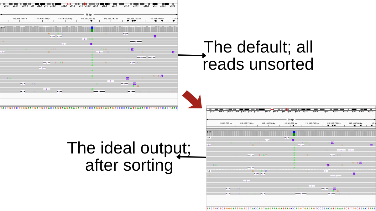
An IGVshot of a genomic region with a C>A base change showing what the reads would look like before and after grouping by base for methylation comparison.

The hard part: structural variants

Structural variants did not earn the label “problematic” for nothing.

As of writing, there are 5 SV types in terms of how they are represented in a VCF: insertions, deletions, duplications, inversions, and breakends. The difficulty is that, unlike an SNV, an SV is not a single-position event you can resolve by reading one base. It is a rearrangement, and finding it on the reads means reasoning about alignment structure.

So let’s take a detour into alignment structure, and something called the CIGAR string, on which SVs lean heavily.

When a read is aligned to the reference genome, the alignment is rarely a clean one-to-one correspondence. Bases get inserted, deleted, clipped. The CIGAR string describes exactly how a read aligns with the reference. It is a string of length-and-operations pairs, read left to right, numbers before letters. Operations (letters) indicate whether bases matched, were inserted, deleted, clipped, skipped, and so on.

A CIGAR like “60M10I35M5D60M” says: 60 bases align to the reference (M), then 10 bases are inserted relative to the reference (I), then 35 align (another M), then 5 reference bases are deleted (D), then 60 more align (another M). M covers both matches and mismatches; it means “aligned,” not “identical”, which is why a C>A substitution does not get its own CIGAR operation but is counted as part of an M. Soft clips (S) appear at read ends where bases were sequenced but not aligned.

Something I initially struggled with here is what each operation consumes, probably because of the choice of word used. Anywho, some operations advance your position along the reference; some advance your position along the read; some do both. M advances both. An insertion (I) advances only the read; that is, those bases are not part of the reference but are on the read, so the reference coordinate stays put. A deletion advances only the reference; that is, the bases exist in the reference but not in this read. This concept is usually phrased as “consumes reference” and “consumes query,” where query is the read, and it lets you walk through a CIGAR while knowing how far into the read you are and which genomic coordinate you are standing on.

Again, I used pysam to access the CIGAR with the cigartuples function, which returns a list of (operation, length) pairs, so one can step through it in a simple loop.

Insertions and deletions

Now, back to parsing the SVs. An insertion is a block of nucleotide bases that appears in the sample at a position where the reference has nothing; a deletion is a block of reference bases that the sample has lost compared to the reference. Both appear within a single linear alignment, so they are visible directly in the CIGAR string.

So, using the cigartuples and the consumes-reference, I could track my position in both coordinate systems (read and reference) and watch for an I or a D operation. A hit, for my purposes, would be an operation whose length matches the SV length in the VCF and whose position matches the VCF position. The same logic serves both insertions and deletions; only the operation letter changes.

Another detour: the SA tag

The remaining SV types cannot be read off a single linear alignment, so before continuing, I need to introduce the SA tag.

When a read spans a rearrangement breakpoint, the aligner often cannot map it as one continuous piece. Instead, it splits the read: one primary alignment and one or more supplementary alignments, each covering a different part of the read. BAM files encode each supplementary piece with the SA tag. For each one, the tag provides its chromosome, position, strand orientation (forward or reverse), CIGAR, and mapping quality. In English, the SA tag says, “this read also aligns somewhere else, and here are the details.”

I didn’t need this for insertions and deletions. However, for inversions, duplications, and breakends, the SA tag is required because the signature of those events is precisely a read that had to be broken across two alignments.

Inversions and duplications

An inversion is a block of bases flipped to the opposite orientation; a duplication is a block amplified in the same orientation. Both have a start point, which is the breakpoint where the read stops matching the reference as expected.

For these, I used the CIGAR on the SA tag rather than the primary CIGAR, and I applied the same length-and-chromosome matching as before, with one addition: strand orientation. The strand sign of the supplementary alignment is the discriminator. If I am looking for a duplication and the supplementary strand matches the reference orientation, that read is a hit. If I am looking for an inversion and the supplementary strand is opposite to the reference, that read is a hit. So the workflow is chromosome matching, position matching, length validation, and strand comparison.

Breakends

A breakend is the same idea as an inversion or a duplication, except the displaced block comes from an entirely different chromosome. So in the SA tag I am no longer matching length at all. I am explicitly looking for a supplementary alignment on the chromosome identified in the VCF. This is also where my tool leans hardest on the VCF being standardised: breakends are encoded with a rigid bracket notation that names the mate position, and my parsing assumes that notation holds. Every. Single. Time.

The unavoidable problem with SVs

You could read all of the above and conclude that SVs, while trickier than SNVs, are still basically straightforward. You would be right, but only for 2 seconds, because…it is not always clear where an SV starts or how long it is.

The VCF gives one position and one length. The reads do not always agree. The same insertion can be recorded at position 18 in the VCF and appear at position 16 on a handful of reads; a variant recorded as 235 bp in length can show up as 240 bp on some reads and exactly 235 on others. This means I had to decide how much wiggle room to allow for each variable, knowing that too much slack will mess with specificity and too little will mess with sensitivity.

I did not find a serious downside to being strict on position, so I was for most SVs, allowing only ±1 bp difference. This means for an insertion/deletion recorded to be on position 18 in the VCF, my code will only find reads where the variant starts at positions 17,18, or 19. I treated length a bit more leniently, allowing roughly ±10 bp, so a 235 bp variant that reads as 240 on one read at the correct position still counts. The wiggle room was not uniform across SV types. For breakends, I loosened the position tolerance to ±10 as well, because at full strictness, I almost never recovered enough supporting reads, and realistically, what are the odds that a genuine chromosomal break lands at the exact same coordinate on every single read?

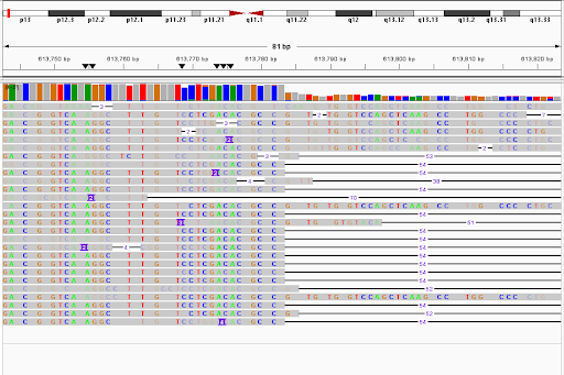
An example of the “problem” with SVs. This is a deletion labelled as 54 bp in the VCF file, starting at the midpoint of the image. But as you can see, not all deletions in this region are 54 bp long, and they don’t all start at the same position. The strictest decision would be to focus on exact matches, but there’ll always be a nagging what if feeling. E.g., What if the 53bp/52bp have the exact same effect but were misaligned?

There is no standard rule for any of this. The wiggle room came out of repeated manual inspections with IGV at different strictness levels. So I made a documented judgment call. It would be convenient to blame the inconsistencies on variant callers and sequence aligners, but that would mean ignoring the 90-or-so percent of positions and lengths they get right. The more honest conclusion is the simple one: SVs are just problematic.

Lessons learned

The result of this endeavour was a working, novel framework for read-based variant–methylation analysis. I learned, in concrete detail, why structural variants resist clean handling. I got to appreciate the beauty of shared standards because, without them, the outcome of this project would be too heavily restricted to certain input formats to be considered widely useful. I learned a great deal about pysam, both its surface and its edges. And I learned the value of building toward a minimum viable version rather than chasing a perfect one. A pipeline that handles SNVs and the tractable SVs correctly, with documented tolerances, is worth more than an unfinished pursuit of absolute perfection that produces nothing to defend. Perhaps most of all, I learned to make decisions without a giant to stand on and to make them defensible, rather than waiting for a certainty that was never going to arrive.

There is also something strangely satisfying about reaching the point where BAM and VCF files stop looking like foreign genomics artefacts.

Resources:

• Samtools tags: https://samtools.github.io/hts-specs/SAMtags.pdf
• Explanation of BAM file content, including CIGAR: PDF documentation of SAM/BAM files.
• VCF file explainer: https://samtools.github.io/hts-specs/VCFv4.4.pdf