Bayesian Reasoning — Soft XOR & Bayesian Networks
I’m perusing this book on Bayesian Reasoning and Machine Learning, freely available online as part of a course on Probabilistic Graphical…
Bayesian Reasoning — Soft XOR & Bayesian Networks
I’m perusing this book on Bayesian Reasoning and Machine Learning, freely available online as part of a course on Probabilistic Graphical Models (CS 228) and along the way examines the soft XOR.

Spotlight on the soft XOR
This example illustrates the difference between the standard XOR and the “soft” version of the XOR. As usual, I will model this with a Bayesian network. I use Netica (but there are others).
Let’s see how this works. Consider the XOR logic gate:

This is easily modeled with Netica

We can use the built-in XOR. The blue node is deterministic.

The truth table for the XOR
Let’s see this simple network in action (the nodes turn green when activated). Notice that once we activate the XOR (by setting it to true), it acts like a constraint on A and B, so whenever A is true, then B is false and vice versa.

Notice that the network is bidirectional
Notice that the XOR gives very crisp boundaries, everything being either true or false. But sometimes we don’t want crisp all-or-nothing boundaries and need to consider fuzzier and less certain outcomes.
Consider, then, a “soft” version of the XOR gate.

Here is the detailed question (and the manually computed answer):

The question: what is p(A = 1 | C = 0)?
This example is worked out much more tediously using BRML on MATLAB (on YouTube). But using a graphical network like Netica is much easier and much faster than text-based systems! We want to avoid manually doing those equations above!
We can reuse our XOR network to build a “soft” XOR:

The generic network with uniform probabilities by default
The tables of interest we could fill manually or with simple equations:

Tables to be filled in manually or with an equation
P (A | ) = .65          // prior for A1

P (B | ) = .77          // prior for B1

P (C | A, B) =          // use state index

      select0 ( 2*A + B, .10, .99, .80, .25)     // maps A, B to prob.
We use the select0 function (above) to map each state index to the corresponding probabilities.
Once the equations are compiled, we have the updated tables for the priors and the likelihood function:

Notice that on each row of C is a conditional probability distribution instead of a truth table
And the updated network:

The updated probabilties for the network
Now, recall the question: what is p (A = 1 | C = 0)? (meaning C is false) :

P( (A = 1 | C = 0) = ~84.4%

The more exact value (ctrl B in netica)
Notice the columnslums in the table for C do not add up to 1:

We can say that this is the likelihood function used in ordercomputeuter the posterior P (C | A, B).
Lets compare and contrast side by side the XOR with the soft XOR. Note that the XOR node is fully deterministic (colored blue).

Notice that the XOR gives crisp true/false answers while the soft XOR gives fuzzier answers
Next time, we will compare and contrast the soft XOR with the Noisy-OR.
REFERENCES
[embed]CS 228 - Probabilistic Graphical Models Winter 2023-24ermongroup.github.io
[embed]https://www.youtube.com/watch?v=cg9JJzHHJQA&list=PL80tEuJBQJYN3NlIKGswYi8x5N4o-0GP4&index=12
메타데이터
- post_id
- 6d1c66eb4750
- slug
- bayesian-reasoning-soft-xor-bayesian-networks-6d1c66eb4750
- url
- https://medium.com/@pbercker/bayesian-reasoning-soft-xor-bayesian-networks-6d1c66eb4750
- canonical_url
- https://medium.com/@pbercker/bayesian-reasoning-soft-xor-bayesian-networks-6d1c66eb4750
- author_url
- https://medium.com/@pbercker
- status
- ok
- fetched_at
- 2026-06-09 15:37:30